
 Topics
excel
Practical Excel skills sharing: Determine whether a cell contains specific content
Topics
excel
Practical Excel skills sharing: Determine whether a cell contains specific content
Practical Excel skills sharing: Determine whether a cell contains specific content

Determining whether a cell contains specified content in Excel is already a commonplace topic. I believe everyone has encountered many similar problems at work. Today I’m going to tell you three common ways to solve this kind of problem, and I’m sure they will work!

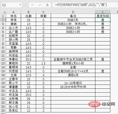
Determining whether a cell contains specific content is a type of problem that is often encountered in daily work. It is common in tables containing remark information. For example, in the attendance summary table below, it is necessary to determine whether the employee works overtime based on the content in the remarks, which falls into this type of problem.

#How to deal with this kind of problem? There are three commonly used formula methods. Let’s introduce them one by one below.
Method 1: IF COUNTIF
Formula: =IF(COUNTIF(D2,"*overtime*")=0, "","Yes")

Formula analysis:
COUNTIF(D2,"*overtime *") is the core part of this formula. This function mainly implements the conditional counting function. The basic format is COUNTIF (conditional area, condition).
In this example, the condition area is a cell "D2", and the condition is the value obtained by adding the wildcard character * on both sides of the content to be judged. The effect is to target cells that meet the condition. The cells are counted. If the content to be judged is included, the result is 1. If it is not included, the result is 0.
After having this result, use the IF function to get the final result, the formula =IF(COUNTIF(D2,"*overtime*")=0,"", "Yes") is easy to understand. If cell D2 does not contain "overtime", the result of COUNTIF is 0, and IF returns the corresponding null value, otherwise it returns "yes".
Let’s look at the second method.
Method 2: IF ISERR FIND
Formula: =IF(ISERR(FIND("Overtime",D2)), "","Yes")
Formula analysis:
The core part of this formula is FIND("Overtime ", D2), the basic format of the FIND function is FIND (what you are looking for, where to find it, and which character to start looking for). If the third parameter is not written, it means starting from the first character. The meaning of this formula is to find the word "overtime" in cell D2. If it can be found, FIND will return the location of the content you are looking for in the cell. If it cannot find it, it will return an error value.

The effect of the FIND function can be seen from the above figure. Next, you need to determine whether the result is an error value. If it is an error value, it means that there is no content you are looking for, so you need to use the ISERR function. The ISERR function is very simple, it just determines whether a value is an error value other than #N/A. In this example, the error value is #VALUE!, so there is no problem using this function.

Finally, add the IF function to form a complete formula =IF(ISERR(FIND("Overtime",D2)),"","Yes") .
Compared with the first method, this formula is slightly more difficult, but it is a good thing to practice the two functions more.
Finally let’s look at the third method.
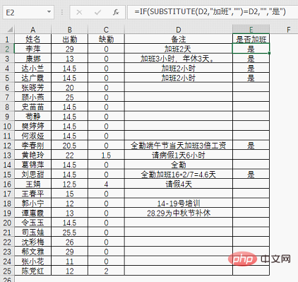
Method 3: IF SUBSTITUTE
Formula: =IF(SUBSTITUTE(D2,"Overtime","")=D2 ,"","Yes")
Formula analysis:
This formula uses a relatively long Function SUBSTITUTE. The function of this function is to replace characters. The format is SUBSTITUTE (where to replace, what to replace, what to replace, and what number to replace). If the last parameter is not written, it means all replacements.
FormulaSUBSTITUTE(D2,"overtime","")means to replace the word "overtime" in cell D2 with nothing. The result after replacement is as shown in the figure Show.

The next step is more interesting. Compare the replaced content with the original content, that is, SUBSTITUTE(D2,"overtime","")=D2. If overtime is included, the replaced content is definitely not equal to The original cell is replaced. On the contrary, if the replaced content is the same as the original content, it means that it does not contain the content you are looking for. In the end, IF is used to output the result.
Compared with the first two methods, the formula =IF(SUBSTITUTE(D2,"overtime","")=D2,"","Yes") is very clever and also Let us re-understand the SUBSTITUTE function from another aspect.
Summary: From the perspective of solving the problem, the first method is sufficient, easy to understand, and relatively simple. But from a learning perspective, when we encounter a problem, we might as well try a few more ideas. On the one hand, we can expand our thinking, and on the other hand, we can become more familiar with some functions. With different solutions, we can also You can experience the fun of studying formula functions. Many so-called masters actually practiced this way.
Related learning recommendations: excel tutorial
The above is the detailed content of Practical Excel skills sharing: Determine whether a cell contains specific content. For more information, please follow other related articles on the PHP Chinese website!

Hot AI Tools

Undresser.AI Undress
AI-powered app for creating realistic nude photos

AI Clothes Remover
Online AI tool for removing clothes from photos.

Undress AI Tool
Undress images for free

Clothoff.io
AI clothes remover

AI Hentai Generator
Generate AI Hentai for free.

Hot Article
Hot Tools

Notepad++7.3.1
Easy-to-use and free code editor

SublimeText3 Chinese version
Chinese version, very easy to use

Zend Studio 13.0.1
Powerful PHP integrated development environment

Dreamweaver CS6
Visual web development tools

SublimeText3 Mac version
God-level code editing software (SublimeText3)
Hot Topics


 How to filter more than 3 keywords at the same time in excel
Mar 21, 2024 pm 03:16 PM
How to filter more than 3 keywords at the same time in excel
Mar 21, 2024 pm 03:16 PM
Excel is often used to process data in daily office work, and it is often necessary to use the "filter" function. When we choose to perform "filtering" in Excel, we can only filter up to two conditions for the same column. So, do you know how to filter more than 3 keywords at the same time in Excel? Next, let me demonstrate it to you. The first method is to gradually add the conditions to the filter. If you want to filter out three qualifying details at the same time, you first need to filter out one of them step by step. At the beginning, you can first filter out employees with the surname "Wang" based on the conditions. Then click [OK], and then check [Add current selection to filter] in the filter results. The steps are as follows. Similarly, perform filtering separately again
 What should I do if the frame line disappears when printing in Excel?
Mar 21, 2024 am 09:50 AM
What should I do if the frame line disappears when printing in Excel?
Mar 21, 2024 am 09:50 AM
If when opening a file that needs to be printed, we will find that the table frame line has disappeared for some reason in the print preview. When encountering such a situation, we must deal with it in time. If this also appears in your print file If you have questions like this, then join the editor to learn the following course: What should I do if the frame line disappears when printing a table in Excel? 1. Open a file that needs to be printed, as shown in the figure below. 2. Select all required content areas, as shown in the figure below. 3. Right-click the mouse and select the "Format Cells" option, as shown in the figure below. 4. Click the “Border” option at the top of the window, as shown in the figure below. 5. Select the thin solid line pattern in the line style on the left, as shown in the figure below. 6. Select "Outer Border"
 How to type subscript in excel
Mar 20, 2024 am 11:31 AM
How to type subscript in excel
Mar 20, 2024 am 11:31 AM
eWe often use Excel to make some data tables and the like. Sometimes when entering parameter values, we need to superscript or subscript a certain number. For example, mathematical formulas are often used. So how do you type the subscript in Excel? ?Let’s take a look at the detailed steps: 1. Superscript method: 1. First, enter a3 (3 is superscript) in Excel. 2. Select the number "3", right-click and select "Format Cells". 3. Click "Superscript" and then "OK". 4. Look, the effect is like this. 2. Subscript method: 1. Similar to the superscript setting method, enter "ln310" (3 is the subscript) in the cell, select the number "3", right-click and select "Format Cells". 2. Check "Subscript" and click "OK"
 How to change excel table compatibility mode to normal mode
Mar 20, 2024 pm 08:01 PM
How to change excel table compatibility mode to normal mode
Mar 20, 2024 pm 08:01 PM
In our daily work and study, we copy Excel files from others, open them to add content or re-edit them, and then save them. Sometimes a compatibility check dialog box will appear, which is very troublesome. I don’t know Excel software. , can it be changed to normal mode? So below, the editor will bring you detailed steps to solve this problem, let us learn together. Finally, be sure to remember to save it. 1. Open a worksheet and display an additional compatibility mode in the name of the worksheet, as shown in the figure. 2. In this worksheet, after modifying the content and saving it, the dialog box of the compatibility checker always pops up. It is very troublesome to see this page, as shown in the figure. 3. Click the Office button, click Save As, and then
 How to set superscript in excel
Mar 20, 2024 pm 04:30 PM
How to set superscript in excel
Mar 20, 2024 pm 04:30 PM
When processing data, sometimes we encounter data that contains various symbols such as multiples, temperatures, etc. Do you know how to set superscripts in Excel? When we use Excel to process data, if we do not set superscripts, it will make it more troublesome to enter a lot of our data. Today, the editor will bring you the specific setting method of excel superscript. 1. First, let us open the Microsoft Office Excel document on the desktop and select the text that needs to be modified into superscript, as shown in the figure. 2. Then, right-click and select the "Format Cells" option in the menu that appears after clicking, as shown in the figure. 3. Next, in the “Format Cells” dialog box that pops up automatically
 How to use the iif function in excel
Mar 20, 2024 pm 06:10 PM
How to use the iif function in excel
Mar 20, 2024 pm 06:10 PM
Most users use Excel to process table data. In fact, Excel also has a VBA program. Apart from experts, not many users have used this function. The iif function is often used when writing in VBA. It is actually the same as if The functions of the functions are similar. Let me introduce to you the usage of the iif function. There are iif functions in SQL statements and VBA code in Excel. The iif function is similar to the IF function in the excel worksheet. It performs true and false value judgment and returns different results based on the logically calculated true and false values. IF function usage is (condition, yes, no). IF statement and IIF function in VBA. The former IF statement is a control statement that can execute different statements according to conditions. The latter
 Where to set excel reading mode
Mar 21, 2024 am 08:40 AM
Where to set excel reading mode
Mar 21, 2024 am 08:40 AM
In the study of software, we are accustomed to using excel, not only because it is convenient, but also because it can meet a variety of formats needed in actual work, and excel is very flexible to use, and there is a mode that is convenient for reading. Today I brought For everyone: where to set the excel reading mode. 1. Turn on the computer, then open the Excel application and find the target data. 2. There are two ways to set the reading mode in Excel. The first one: In Excel, there are a large number of convenient processing methods distributed in the Excel layout. In the lower right corner of Excel, there is a shortcut to set the reading mode. Find the pattern of the cross mark and click it to enter the reading mode. There is a small three-dimensional mark on the right side of the cross mark.
 How to insert excel icons into PPT slides
Mar 26, 2024 pm 05:40 PM
How to insert excel icons into PPT slides
Mar 26, 2024 pm 05:40 PM
1. Open the PPT and turn the page to the page where you need to insert the excel icon. Click the Insert tab. 2. Click [Object]. 3. The following dialog box will pop up. 4. Click [Create from file] and click [Browse]. 5. Select the excel table to be inserted. 6. Click OK and the following page will pop up. 7. Check [Show as icon]. 8. Click OK.
