Practical Excel skills sharing: Find the maximum and minimum values ​​​​according to conditions!

Speaking of finding the maximum and minimum values ​​​​according to conditions in excel, what do you usually do? Some students may say, use the new functions MAXIFS and MINIFS. Indeed, these two functions updated in the OFFICE 365 subscription version and OFFICE 2019 can directly solve the problem. However, the OFFICE 365 subscription version is charged annually, and OFFICE 2019 can only be installed on the WIN 10 operating system, which feels quite restrictive. So besides these two functions, are there any other methods? Follow the editor and take a look below!

One day, an old classmate who was a teacher called...

"I have a question to ask you. I'm almost crazy with my work. I am counting the scores of the whole school. Now I want to count the highest and lowest scores of each class. There are 12 classes in one grade, and there are 72 classes in 6 grades. All students are in one table, and they are also divided into Chinese, Mathematics and English."

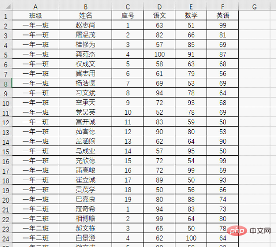
"I know that you can use the MAX and MIN functions to find the highest and lowest scores, but if you want to calculate the highest and lowest scores for each class , I need to use these two functions one by one, please help me and treat you to dinner."

"What version of Excel are you using?"

"It's 2019. "

"That's easy to handle. There are several new functions in office 2019 and office 365 subscription versions. Your problem can be solved with the new functions."

"Then tell me quickly. Say."

"These two functions are MAXIFS and MINIFS."

"I have never seen this before. I have only seen COUNTIFS and SUMIFS."

"Actually The usage of these two functions is really similar to SUMIFS. Let me give you two simple examples."

Now we want to return the highest and lowest scores of the "Chinese" subject in different classes, the formula is:

=MAXIFS(D:D,$A:$A,$I3)
=MINIFS(D:D,$A:$A,$I3)

The results are shown in the figure.

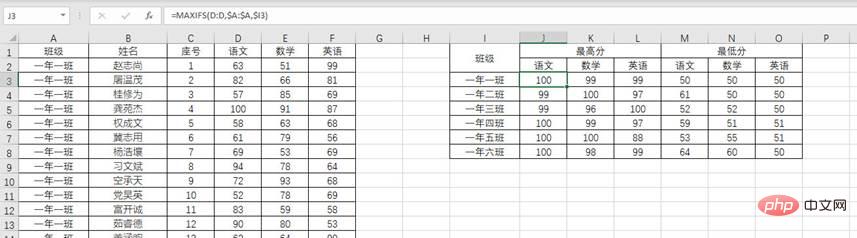
The "$" is used in the formula to fix the area and prevent the area in the formula from shifting when pulling to the right.

Here is a brief introduction to these two new functions. Take the MAXIFS function as an example. Its function is to return the maximum value that satisfies all conditions in the area. The function structure is =MAXIFS (specified area, condition area, condition). Back to the formula, =MAXIFS(D:D,$A:$A,$I3) means to find the data in column A that meets the conditions of cell I3 and return the maximum value in the corresponding data in column D. . (MINIFS function structure is similar.)

"Use these two functions to directly get the results you want."

"Then what should I do if I encounter similar problems in school? Do it, the school's office version does not support these two functions!"

"This is easy to do, but it is a little troublesome. I will teach you a few more methods."

① Array function

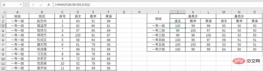
Before the emergence of MAXIFS and MINIFS functions, most array functions were used to solve this problem.

=MAX(IF($A:$A= $I3,D:D))
=MIN(IF($A:$A= $I3,D:D))

After inputting the array function, you must use the CTRL SHINF ENTER three keys to end the input. You cannot directly press the Enter key to end the input. And after the formula is entered, a layer of braces will be placed around the outermost part of the function. Entering curly braces directly has no effect.

"Array function, this seems quite difficult. Is there an easier way?"

② Pivot table

"If the array function still feels troublesome, then use a pivot table to solve it."

"I know the pivot table. Just pull it and it will be fine. It's just me. Remember that pivot tables are used for summing."

"Pivot tables have more than just summing functions. Let me show you how to operate them."

First of all, according to the figure below, Display to create a PivotTable.

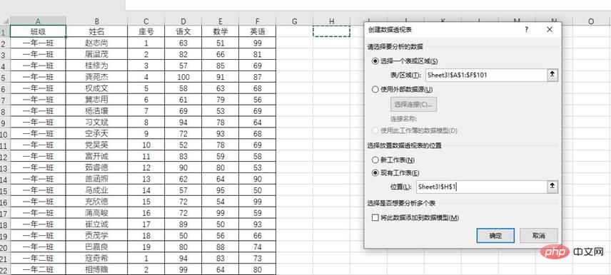
Then set the corresponding "row" and "column" data, put "class" under the "row" label, "Chinese", "Mathematics", "English" is placed under the "Values" tag. Place the three account data again.

Now comes the most critical step, change the summation item in the field to the maximum value or minimum value.

"After learning these tricks, you can easily solve this kind of problem again."

"But I still ask you to help me. The fastest processing╰(￣▽￣)╭”

“You...

Related learning recommendations: excel tutorial

The above is the detailed content of Practical Excel skills sharing: Find the maximum and minimum values ​​​​according to conditions!. For more information, please follow other related articles on the PHP Chinese website!