
 Technology peripherals
AI
'In-depth Analysis': Exploring LiDAR Point Cloud Segmentation Algorithm in Autonomous Driving
Technology peripherals
AI
'In-depth Analysis': Exploring LiDAR Point Cloud Segmentation Algorithm in Autonomous Driving
'In-depth Analysis': Exploring LiDAR Point Cloud Segmentation Algorithm in Autonomous Driving

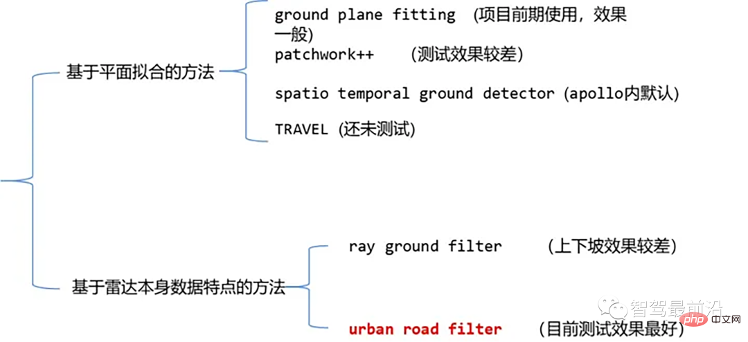
Currently, the common laser point cloud segmentation algorithms include methods based on plane fitting and methods based on the characteristics of laser point cloud data. The details are as follows:
Point cloud ground segmentation algorithm
01 Based on plane Fitting method - Ground Plane Fitting
Algorithm idea: A simple processing method is to divide the space into several sub-planes along the x direction (the direction of the car head), and then perform each The sub-plane uses the ground plane fitting algorithm (GPF) to obtain a ground segmentation method that can handle steep slopes. This method is to fit a global plane in a single frame point cloud. It works better when the number of point clouds is large. When the point cloud is sparse, it is easy to cause missed detections and false detections, such as 16-line lidar.
Algorithm pseudo code:
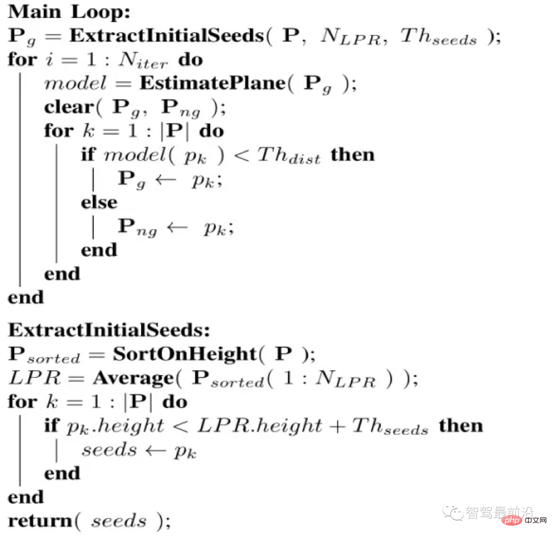
Pseudo code
The algorithm process is that for a given point cloud P, the final result of segmentation is two point cloud collections, ground point clouds and non-ground point clouds. This algorithm has four important parameters, as follows:
- Niter: the number of times to perform singular value decomposition (SVD), that is, the number of times to perform optimization fitting
- NLPR: The number of lowest height points used to select LPR
- Thseed: The threshold used to select seed points, when the height of the point in the point cloud is less than When the height of LPR is added to this threshold, we add the point to the seed point set
- Thdist: Plane distance threshold, we will calculate each point in the point cloud to the plane we fit. The distance of the orthogonal projection, and this plane distance threshold is used to determine whether the point belongs to the ground
Selection of seed point set
We first select a seed point set (seed point set). These seed points are derived from points with smaller height (i.e. z value) in the point cloud. The seed point set is used to establish an initial plane model describing the ground, then How to select this seed point set? We introduce the concept of Lowest Point Representative (LPR). LPR is the average of the lowest height points of NLPR. LPR ensures that the plane fitting stage is not affected by measurement noise.
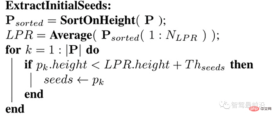
Selection of seed points
The input is a frame of point cloud, The points in this point cloud have been sorted along the z direction (i.e., height). Take num_lpr_ minimum points, find the height average lpr_height (i.e., LPR), and select points with a height less than lpr_height th_seeds_ as seed points.
The specific code is implemented as follows
/*
@brief Extract initial seeds of the given pointcloud sorted segment.
This function filter ground seeds points accoring to heigt.
This function will set the `g_ground_pc` to `g_seed_pc`.
@param p_sorted: sorted pointcloud

@param ::num_lpr_: num of LPR points
@param ::th_seeds_: threshold distance of seeds
@param ::
*/
void PlaneGroundFilter::extract_initial_seeds_(const pcl::PointCloud &p_sorted)
{
// LPR is the mean of low point representative
double sum = 0;
int cnt = 0;
// Calculate the mean height value.
for (int i = 0; i Flat model
Connect Next, we build a plane model. If the orthogonal projection distance of a point in the point cloud to this plane is less than the threshold Thdist, the point is considered to belong to the ground, otherwise it belongs to the non-ground. A simple linear model is used for plane model estimation, as follows:
ax by cz d=0
That is:
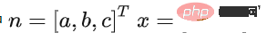
is calculated by the covariance matrix C of the initial point set Solve for n to determine a plane. The seed point set is used as the initial point set, and its covariance matrix is
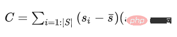
这个协方差矩阵 C 描述了种子点集的散布情况,其三个奇异向量可以通过奇异值分解(SVD)求得,这三个奇异向量描述了点集在三个主要方向的散布情况。由于是平面模型,垂直于平面的法向量 n 表示具有最小方差的方向,可以通过计算具有最小奇异值的奇异向量来求得。
那么在求得了 n 以后, d 可以通过代入种子点集的平均值 ,s(它代表属于地面的点) 直接求得。整个平面模型计算代码如下:
/*
@brief The function to estimate plane model. The
model parameter `normal_` and `d_`, and `th_dist_d_`
is set here.
The main step is performed SVD(UAV) on covariance matrix.
Taking the sigular vector in U matrix according to the smallest
sigular value in A, as the `normal_`. `d_` is then calculated
according to mean ground points.


@param g_ground_pc:global ground pointcloud ptr.

*/
void PlaneGroundFilter::estimate_plane_(void)
{
// Create covarian matrix in single pass.
// TODO: compare the efficiency.
Eigen::Matrix3f cov;
Eigen::Vector4f pc_mean;
pcl::computeMeanAndCovarianceMatrix(*g_ground_pc, cov, pc_mean);
// Singular Value Decomposition: SVD
JacobiSVD svd(cov, Eigen::DecompositionOptions::ComputeFullU);
// use the least singular vector as normal
normal_ = (svd.matrixU().col(2));
// mean ground seeds value
Eigen::Vector3f seeds_mean = pc_mean.head();


// according to normal.T*[x,y,z] = -d
d_ = -(normal_.transpose() * seeds_mean)(0, 0);
// set distance threhold to `th_dist - d`
th_dist_d_ = th_dist_ - d_;


// return the equation parameters
}优化平面主循环
extract_initial_seeds_(laserCloudIn);
g_ground_pc = g_seeds_pc;
// Ground plane fitter mainloop
for (int i = 0; i clear();
g_not_ground_pc->clear();


//pointcloud to matrix
MatrixXf points(laserCloudIn_org.points.size(), 3);
int j = 0;
for (auto p : laserCloudIn_org.points)
{
points.row(j++) points.push_back(laserCloudIn_org[r]);
}
}
}得到这个初始的平面模型以后,我们会计算点云中每一个点到该平面的正交投影的距离,即 points * normal_,并且将这个距离与设定的阈值(即th_dist_d_) 比较,当高度差小于此阈值,我们认为该点属于地面,当高度差大于此阈值,则为非地面点。经过分类以后的所有地面点被当作下一次迭代的种子点集,迭代优化。
02 基于雷达数据本身特点的方法-Ray Ground Filter
代码
https://www.php.cn/link/a8d3b1e36a14da038a06f675d1693dd8
算法思想
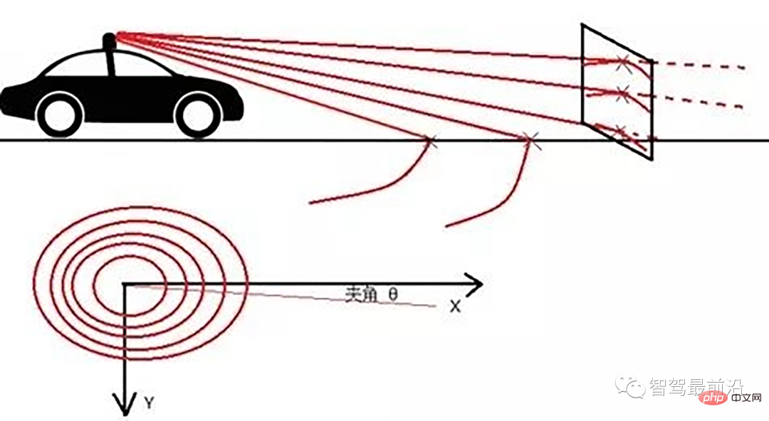
Ray Ground Filter算法的核心是以射线(Ray)的形式来组织点云。将点云的 (x, y, z)三维空间降到(x,y)平面来看,计算每一个点到车辆x正方向的平面夹角 θ, 对360度进行微分,分成若干等份,每一份的角度为0.2度。
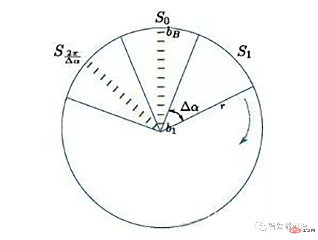
激光线束等间隔划分示意图(通常以激光雷达角度分辨率划分)
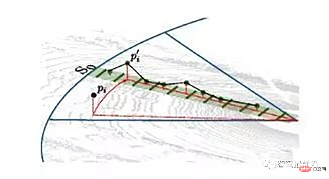
同一角度范围内激光线束在水平面的投影以及在Z轴方向的高度折线示意图
为了方便对同一角度的线束进行处理,要将原来直角坐标系的点云转换成柱坐标描述的点云数据结构。对同一夹角的线束上的点按照半径的大小进行排序,通过前后两点的坡度是否大于我们事先设定的坡度阈值,从而判断点是否为地面点。
线激光线束纵截面与俯视示意图(n=4)
通过如下公式转换成柱坐标的形式:
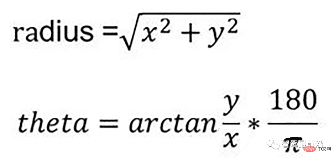
转换成柱坐标的公式
radius表示点到lidar的水平距离(半径),theta是点相对于车头正方向(即x方向)的夹角。对点云进行水平角度微分之后,可得到1800条射线,将这些射线中的点按照距离的远近进行排序。通过两个坡度阈值以及当前点的半径求得高度阈值,通过判断当前点的高度(即点的z值)是否在地面加减高度阈值范围内来判断当前点是为地面。
伪代码

伪代码
- local_max_slope_ :设定的同条射线上邻近两点的坡度阈值。
- general_max_slope_ :整个地面的坡度阈值
遍历1800条射线,对于每一条射线进行如下操作:
1.计算当前点和上一个点的水平距离pointdistance
2.根据local_max_slope_和pointdistance计算当前的坡度差阈值height_threshold
3.根据general_max_slope_和当前点的水平距离计算整个地面的高度差阈值general_height_threshold
4.若当前点的z坐标小于前一个点的z坐标加height_threshold并大于前一个点的z坐标减去height_threshold:
5.若当前点z坐标小于雷达安装高度减去general_height_threshold并且大于相加,认为是地面点
6.否则:是非地面点。
7.若pointdistance满足阈值并且前点的z坐标小于雷达安装高度减去height_threshold并大于雷达安装高度加上height_threshold,认为是地面点。
/*!
 *
 * @param[in] in_cloud Input Point Cloud to be organized in radial segments
 * @param[out] out_organized_points Custom Point Cloud filled with XYZRTZColor data
 * @param[out] out_radial_divided_indices Indices of the points in the original cloud for each radial segment
 * @param[out] out_radial_ordered_clouds Vector of Points Clouds, each element will contain the points ordered
 */
void PclTestCore::XYZI_to_RTZColor(const pcl::PointCloud::Ptr in_cloud,
 PointCloudXYZIRTColor &out_organized_points,
 std::vector &out_radial_divided_indices,
 std::vector &out_radial_ordered_clouds)
{
out_organized_points.resize(in_cloud->points.size());
out_radial_divided_indices.clear();
out_radial_divided_indices.resize(radial_dividers_num_);
out_radial_ordered_clouds.resize(radial_dividers_num_);

for (size_t i = 0; i points.size(); i++)
{
PointXYZIRTColor new_point;
//计算radius和theta
//方便转到柱坐标下。
auto radius = (float)sqrt(
in_cloud->points[i].x * in_cloud->points[i].x + in_cloud->points[i].y * in_cloud->points[i].y);
auto theta = (float)atan2(in_cloud->points[i].y, in_cloud->points[i].x) * 180 / M_PI;
if (theta points[i];
new_point.radius = radius;
new_point.theta = theta;
new_point.radial_div = radial_div;
new_point.concentric_div = concentric_div;
new_point.original_index = i;

out_organized_points[i] = new_point;

//radial divisions更加角度的微分组织射线
out_radial_divided_indices[radial_div].indices.push_back(i);

out_radial_ordered_clouds[radial_div].push_back(new_point);

} //end for

//将同一根射线上的点按照半径(距离)排序
#pragma omp for
for (size_t i = 0; i 03 基于雷达数据本身特点的方法-urban road filter
原文
Real-Time LIDAR-Based Urban Road and Sidewalk Detection for Autonomous Vehicles
代码
https://www.php.cn/link/305fa4e2c0e76dd586553d64c975a626
z_zero_method
z_zero_method
首先将数据组织成[channels][thetas]
对于每一条线,对角度进行排序
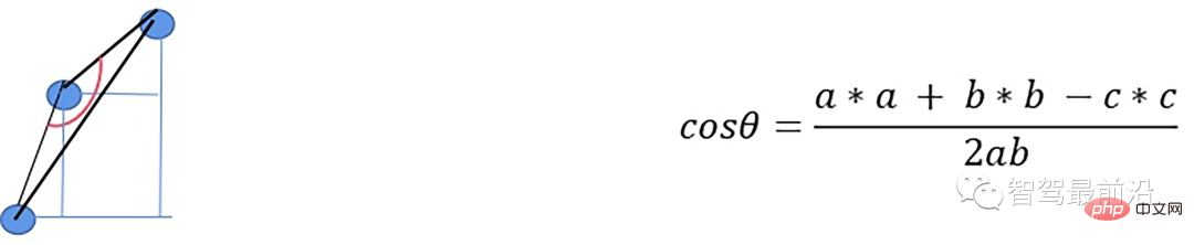
- 以当前点p为中心,向左选k个点,向右选k个点
- 分别计算左边及右边k个点与当前点在x和y方向差值的均值
- 同时计算左边及右边k个点的最大z值max1及max2
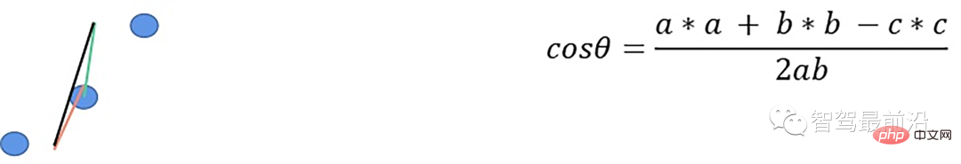
- 根据余弦定理求解余弦角
如果余弦角度满足阈值且max1减去p.z满足阈值或max2减去p.z满足阈值且max2-max1满足阈值,认为此点为障碍物,否则就认为是地面点。
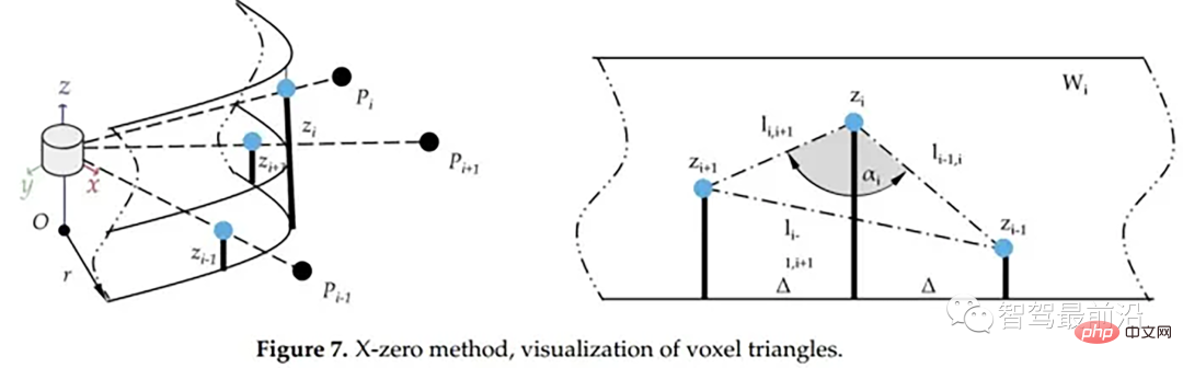
x_zero_method
X-zero和Z-zero方法可以找到避开测量的X和Z分量的人行道,X-zero和Z-zero方法都考虑了体素的通道数,因此激光雷达必须与路面平面不平行,这是上述两种算法以及整个城市道路滤波方法的已知局限性。X-zero方法去除了X方向的值,使用柱坐标代替。
x_zero_method
首先将数据组织成[channels][thetas]
For each line, sort the angles
- With the current point p as the center, select the k/2th point p1 and the kth point p2 to the right
- Calculate the distance in the z direction between p and p1, p1 and p2, p and p2 respectively
- Solve the cosine angle according to the cosine theorem
If the cosine angle meets the threshold and p1.z-p.z meets the threshold or p1.z-p2.z meets the threshold and p.z-p2.z meets the threshold, this point is considered an obstacle
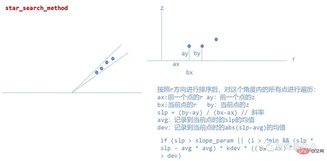
star_search_method
This method divides the point cloud into rectangular segments, the combination of these shapes resembles a star; this is where the name comes from, from each road segments to extract possible sidewalk starting points, the algorithm created therein is insensitive to height changes based on the Z coordinate, which means that in practice the algorithm will perform well even when the lidar is tilted relative to the road surface plane, in cylindrical coordinates The system processes point clouds.
Specific implementation:
##star_search_method
The above is the detailed content of 'In-depth Analysis': Exploring LiDAR Point Cloud Segmentation Algorithm in Autonomous Driving. For more information, please follow other related articles on the PHP Chinese website!

Hot AI Tools

Undresser.AI Undress
AI-powered app for creating realistic nude photos

AI Clothes Remover
Online AI tool for removing clothes from photos.

Undress AI Tool
Undress images for free

Clothoff.io
AI clothes remover

AI Hentai Generator
Generate AI Hentai for free.

Hot Article
Hot Tools

Notepad++7.3.1
Easy-to-use and free code editor

SublimeText3 Chinese version
Chinese version, very easy to use

Zend Studio 13.0.1
Powerful PHP integrated development environment

Dreamweaver CS6
Visual web development tools

SublimeText3 Mac version
God-level code editing software (SublimeText3)
Hot Topics
 1377
1377
 52
52

 Why is Gaussian Splatting so popular in autonomous driving that NeRF is starting to be abandoned?
Jan 17, 2024 pm 02:57 PM
Why is Gaussian Splatting so popular in autonomous driving that NeRF is starting to be abandoned?
Jan 17, 2024 pm 02:57 PM
Written above & the author’s personal understanding Three-dimensional Gaussiansplatting (3DGS) is a transformative technology that has emerged in the fields of explicit radiation fields and computer graphics in recent years. This innovative method is characterized by the use of millions of 3D Gaussians, which is very different from the neural radiation field (NeRF) method, which mainly uses an implicit coordinate-based model to map spatial coordinates to pixel values. With its explicit scene representation and differentiable rendering algorithms, 3DGS not only guarantees real-time rendering capabilities, but also introduces an unprecedented level of control and scene editing. This positions 3DGS as a potential game-changer for next-generation 3D reconstruction and representation. To this end, we provide a systematic overview of the latest developments and concerns in the field of 3DGS for the first time.
 How to solve the long tail problem in autonomous driving scenarios?
Jun 02, 2024 pm 02:44 PM
How to solve the long tail problem in autonomous driving scenarios?
Jun 02, 2024 pm 02:44 PM
Yesterday during the interview, I was asked whether I had done any long-tail related questions, so I thought I would give a brief summary. The long-tail problem of autonomous driving refers to edge cases in autonomous vehicles, that is, possible scenarios with a low probability of occurrence. The perceived long-tail problem is one of the main reasons currently limiting the operational design domain of single-vehicle intelligent autonomous vehicles. The underlying architecture and most technical issues of autonomous driving have been solved, and the remaining 5% of long-tail problems have gradually become the key to restricting the development of autonomous driving. These problems include a variety of fragmented scenarios, extreme situations, and unpredictable human behavior. The "long tail" of edge scenarios in autonomous driving refers to edge cases in autonomous vehicles (AVs). Edge cases are possible scenarios with a low probability of occurrence. these rare events
 Choose camera or lidar? A recent review on achieving robust 3D object detection
Jan 26, 2024 am 11:18 AM
Choose camera or lidar? A recent review on achieving robust 3D object detection
Jan 26, 2024 am 11:18 AM
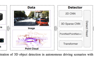
0.Written in front&& Personal understanding that autonomous driving systems rely on advanced perception, decision-making and control technologies, by using various sensors (such as cameras, lidar, radar, etc.) to perceive the surrounding environment, and using algorithms and models for real-time analysis and decision-making. This enables vehicles to recognize road signs, detect and track other vehicles, predict pedestrian behavior, etc., thereby safely operating and adapting to complex traffic environments. This technology is currently attracting widespread attention and is considered an important development area in the future of transportation. one. But what makes autonomous driving difficult is figuring out how to make the car understand what's going on around it. This requires that the three-dimensional object detection algorithm in the autonomous driving system can accurately perceive and describe objects in the surrounding environment, including their locations,
 Have you really mastered coordinate system conversion? Multi-sensor issues that are inseparable from autonomous driving
Oct 12, 2023 am 11:21 AM
Have you really mastered coordinate system conversion? Multi-sensor issues that are inseparable from autonomous driving
Oct 12, 2023 am 11:21 AM
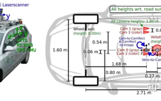
The first pilot and key article mainly introduces several commonly used coordinate systems in autonomous driving technology, and how to complete the correlation and conversion between them, and finally build a unified environment model. The focus here is to understand the conversion from vehicle to camera rigid body (external parameters), camera to image conversion (internal parameters), and image to pixel unit conversion. The conversion from 3D to 2D will have corresponding distortion, translation, etc. Key points: The vehicle coordinate system and the camera body coordinate system need to be rewritten: the plane coordinate system and the pixel coordinate system. Difficulty: image distortion must be considered. Both de-distortion and distortion addition are compensated on the image plane. 2. Introduction There are four vision systems in total. Coordinate system: pixel plane coordinate system (u, v), image coordinate system (x, y), camera coordinate system () and world coordinate system (). There is a relationship between each coordinate system,
 This article is enough for you to read about autonomous driving and trajectory prediction!
Feb 28, 2024 pm 07:20 PM
This article is enough for you to read about autonomous driving and trajectory prediction!
Feb 28, 2024 pm 07:20 PM
Trajectory prediction plays an important role in autonomous driving. Autonomous driving trajectory prediction refers to predicting the future driving trajectory of the vehicle by analyzing various data during the vehicle's driving process. As the core module of autonomous driving, the quality of trajectory prediction is crucial to downstream planning control. The trajectory prediction task has a rich technology stack and requires familiarity with autonomous driving dynamic/static perception, high-precision maps, lane lines, neural network architecture (CNN&GNN&Transformer) skills, etc. It is very difficult to get started! Many fans hope to get started with trajectory prediction as soon as possible and avoid pitfalls. Today I will take stock of some common problems and introductory learning methods for trajectory prediction! Introductory related knowledge 1. Are the preview papers in order? A: Look at the survey first, p
 SIMPL: A simple and efficient multi-agent motion prediction benchmark for autonomous driving
Feb 20, 2024 am 11:48 AM
SIMPL: A simple and efficient multi-agent motion prediction benchmark for autonomous driving
Feb 20, 2024 am 11:48 AM
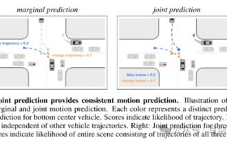
Original title: SIMPL: ASimpleandEfficientMulti-agentMotionPredictionBaselineforAutonomousDriving Paper link: https://arxiv.org/pdf/2402.02519.pdf Code link: https://github.com/HKUST-Aerial-Robotics/SIMPL Author unit: Hong Kong University of Science and Technology DJI Paper idea: This paper proposes a simple and efficient motion prediction baseline (SIMPL) for autonomous vehicles. Compared with traditional agent-cent
 nuScenes' latest SOTA | SparseAD: Sparse query helps efficient end-to-end autonomous driving!
Apr 17, 2024 pm 06:22 PM
nuScenes' latest SOTA | SparseAD: Sparse query helps efficient end-to-end autonomous driving!
Apr 17, 2024 pm 06:22 PM
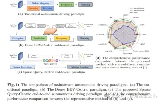
Written in front & starting point The end-to-end paradigm uses a unified framework to achieve multi-tasking in autonomous driving systems. Despite the simplicity and clarity of this paradigm, the performance of end-to-end autonomous driving methods on subtasks still lags far behind single-task methods. At the same time, the dense bird's-eye view (BEV) features widely used in previous end-to-end methods make it difficult to scale to more modalities or tasks. A sparse search-centric end-to-end autonomous driving paradigm (SparseAD) is proposed here, in which sparse search fully represents the entire driving scenario, including space, time, and tasks, without any dense BEV representation. Specifically, a unified sparse architecture is designed for task awareness including detection, tracking, and online mapping. In addition, heavy
 Let's talk about end-to-end and next-generation autonomous driving systems, as well as some misunderstandings about end-to-end autonomous driving?
Apr 15, 2024 pm 04:13 PM
Let's talk about end-to-end and next-generation autonomous driving systems, as well as some misunderstandings about end-to-end autonomous driving?
Apr 15, 2024 pm 04:13 PM
In the past month, due to some well-known reasons, I have had very intensive exchanges with various teachers and classmates in the industry. An inevitable topic in the exchange is naturally end-to-end and the popular Tesla FSDV12. I would like to take this opportunity to sort out some of my thoughts and opinions at this moment for your reference and discussion. How to define an end-to-end autonomous driving system, and what problems should be expected to be solved end-to-end? According to the most traditional definition, an end-to-end system refers to a system that inputs raw information from sensors and directly outputs variables of concern to the task. For example, in image recognition, CNN can be called end-to-end compared to the traditional feature extractor + classifier method. In autonomous driving tasks, input data from various sensors (camera/LiDAR
