
 Technology peripherals
AI
Turing machine is the hottest recurrent neural network RNN in deep learning? The 1996 paper proved it!
Technology peripherals
AI
Turing machine is the hottest recurrent neural network RNN in deep learning? The 1996 paper proved it!
Turing machine is the hottest recurrent neural network RNN in deep learning? The 1996 paper proved it!

The Finnish Artificial Intelligence Conference organized by the Finnish Artificial Intelligence Association and the University of Vaasa was held in Vaasa, Finland from August 19 to 23, 1996.
A paper published at the conference proved that the Turing machine is a recurrent neural network.
Yes, this was 26 years ago!
Let us take a look at this paper published in 1996.
1 Preface
1.1 Neural Network Classification
Neural networks can be used for classification tasks to determine whether the input pattern belongs to a specific category.
It has long been known that single-layer feedforward networks can only be used to classify linearly separable patterns, that is, the more consecutive layers, the more complex the distribution of classes.
When feedback is introduced in the network structure, the perceptron output value is recycled, and the number of consecutive layers becomes infinite in principle.
Has the computing power been qualitatively improved? The answer is yes.
For example, you can construct a classifier to determine whether the input integer is prime.
It turns out that the size of the network used for this purpose can be finite, and even if the input integer size is not limited, the number of primes that can be correctly classified is infinite.
In this article, "a cyclic network structure composed of the same computational elements" can be used to complete any (algorithmically) computable function.
1.2 About computability
According to the basic axioms of computability theory, Turing machines can be used to implement computable functions. There are many ways to implement Turing machines.
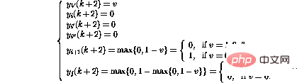
Define programming language . The language has four basic operations:
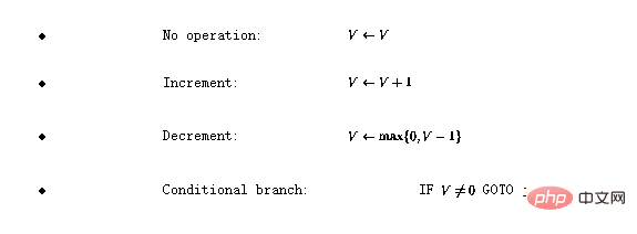
Here, V represents any variable with a positive integer value, j represents any line number.
It can be shown that if a function is Turing computable, it can be encoded using this simple language (see [1] for details) .
2 Turing Network
2.1 Recursive Neural Network Structure
The neural network studied in this article consists of perceptrons, all of which have the same The structure of the perceptron number q can be defined as
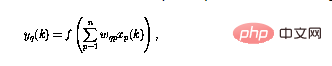
. Among them, the perceptron output at the current moment (using  represents) is calculated using n input
  .
.
Nonlinear function f can now be defined as
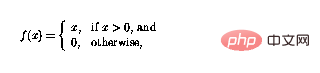
so that the function can Simply "cutting off" negative values, loops in a perceptron network means that perceptrons can be combined in complex ways.
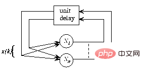
Figure 1 The overall framework of the recurrent neural network, the structure is autonomous without external input, and the network behavior is completely determined by the initial state
In Figure 1 , the recursive structure is shown in a general framework: now  and n are the numbers of perceptrons, and the connection from perceptron p to perceptron q is given by
  Scalar weight representation.
That is, given an initial state, the network state will iterate until it no longer changes, and the results can be read at the stable state or the "fixed point" of the network.
2.2 Neural Network Construction
The following explains how the program is implemented in the perceptron network. The network consists of the following nodes (or perceptrons):
-
For every variable V in the program, there is a variable node
 .
. -
For each program line i, there is an instruction node .
-
For each conditional branch instruction on line i, there are two additional branch nodes and .
 .
.  .
.  and
and  .
. Language The implementation of the program includes the following changes to the perceptron network:
- For the program For each variable in V, use the following link to expand the network:

-
If the program code If there is no operation () on line i, use the following link to expand the network (assuming the node exists:
 , use the following link to expand the network (assuming the node
  exists:
-
If there is an incremental operation () in line i, expand the network as follows:
 , expand the network as follows:
-
If there is a decrement operation () in line i, expand the network as follows:
 , expand the network as follows:
-
If there is a conditional branch () at line i, expand the network as follows:
 , expand the network as follows:
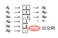
2.3 Equivalence Proof
What needs to be proved now is that "the internal state of the network or the content of the network node" can be identified by the program state, while the network Continuity of state corresponds to program flow.
Define the "legal state" of the network as follows:
-
to all transition nodes and The output of (as defined in 2.2) is zero ();
-
at most one instruction node has a unit output (), all other instruction nodes have a zero output, and the
- variable node has a non-negative integer output value.


If the outputs of all instruction nodes are zero, the state is the final state . A legal network state can be directly interpreted as a program "snapshot" - if , the program counter is at line i, and the corresponding variable value is stored in in the variable node.
Changes in network status are activated by non-zero nodes.
First, focusing on the variable nodes, it turns out that they behave like integrators and the previous contents of the node are looped back to the same node.
The only connections from variable nodes to other nodes have negative weights - that's why nodes containing zeros don't change, because of non-linearity (2).
Next, the instruction node is explained in detail. Assume that the only non-zero instruction node is at time k---this corresponds to the program counter at line i in the program code .
If line i in the program is , then the behavior of the network taking one step forward can be expressed as ( Only affected nodes shown)

It turns out that the new network state is legitimate again. Compared to the program code, this corresponds to the program counter being moved to line i 1.
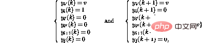
On the other hand, if line i in the program is  , then the behavior of one step forward is
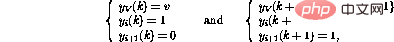
In this way, in addition to moving the program counter to the next line, the value of the variable V will also be decremented. If line i were
 , the operation of the network would be the same except that the value of variable V is increased.
The conditional branch operation (IF GOTO  j) at line i activates a more complex sequence of operations :
##Finally,
It turns out that in these After the step, the network state can again be interpreted as another program snapshot.
The variable value has been changed and the token has been moved to the new location as if the corresponding program line had been executed.
If the token disappears, the network state no longer changes - this can only happen if the program counter "exceeds" the program code, which means the program terminates.
The operation of the network is also similar to the operation of the corresponding program, and the proof is completed.
3 Modification3.1 Extension
It is easy to define additional streamlined instructions that can make programming easier, And the generated program is more readable and executes faster. For example, the unconditional branch (GOTO j) at line
- ## at line
- i can be implemented as
Add the constant c to the variable at line - i () can be implemented as ## Another conditional branch (IF V
=0 GOTO j) on line -
can be achieved For
Additionally, various increment/decrement instructions can be evaluated simultaneously. Suppose you want to perform the following operations: - . Only one node is needed :
The above method is by no means an implementation of a Turing machine the only way.
This is a simple implementation and may not necessarily be optimal in an application.
3.2 Matrix formulation
The above construction can also be implemented in the form of a matrix.
The basic idea is to store the variable value and "program counter" in the process state s, and let the state transition matrix
Arepresent the node links between. The operation of the matrix structure can be defined as a discrete-time dynamic process

where the nonlinear vector-valued function  is now defined element-wise as in (2).
The contents of the state transition matrixA are easily decoded from the network formula - the matrix elements are the weights between nodes.
This matrix formula is similar to the "concept matrix" framework proposed in [3].
4 Example
Suppose you want to implement a simple function y=x, that is, input the value of the variable x Should be passed to the output variable y. Using language  this can be encoded as (so that the "entry point" is now not the first line but the third line):
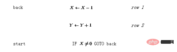
The generated perceptron network is shown in Figure 2.
The solid line represents a positive connection (weight is 1), and the dotted line represents a negative connection (weight is -1). Compared with Figure 1, the network structure is redrawn and simplified by integrating delay elements in the nodes.
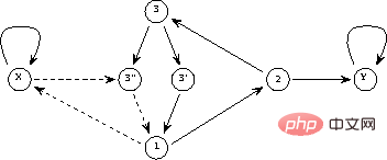
Figure 2 Network implementation of a simple program
In matrix form , the program above would look like
The first two rows/columns in matrix A correspond to the variables connected to represent the two Links to the nodes Y and X, the next three lines represent the three program lines (1, 2, and 3), and the last two represent the additional nodes required for the branch instruction (3 ' and 3'').
Then there are the initial (before iteration) and final (after iteration, when the fixed point is found) states
If the value of the variable node will be kept strictly between 0 and 1, the operation of the dynamic system (3) will be linear and the function will have no effect at all.
In principle, linear systems theory can then be used in the analysis.
For example, in FIG. 3 , the eigenvalues of the state transition matrix A are shown.
Even if there are eigenvalues outside the unit circle in the above example, the nonlinearity makes the iteration always stable.
It turns out that the iteration always converges after  steps, where
  .
.
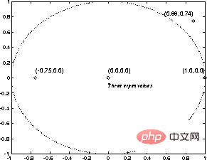
Figure 3 "Characteristic value" of a simple program
5 Discussion
5.1 Theoretical aspects
The results show that Turing machines can be encoded as perceptron networks.
By definition, all computable functions are Turing computable - within the framework of computability theory, no more powerful computational system exists.
This is why, it can be concluded -
The recurrent perceptron network (shown above) is a Turing machine (yet another) form.
The advantage of this equivalence is that the results of computability theory are easy to obtain - for example, given a network and an initial state, it is impossible to judge the process Will it eventually stop.
The above theoretical equivalence does not say anything about computational efficiency.
The different mechanisms that occur in the network can make some functions better implemented in this framework compared to traditional Turing machine implementations (which are actually today's computers).
# At least in some cases, for example, a network implementation of an algorithm can be parallelized by allowing multiple "program counters" in the snapshot vector.
The operation of the network is strictly local, not global.
An interesting question arises, for example, whether the NP-complete problem can be attacked more effectively in a network environment!
Compared to the language , the network implementation has the following "extensions":
-
Variables Can be continuous, not just integer values. In fact, the (theoretical) ability to represent real numbers makes network implementations more powerful than the language , in which all numbers represented are rational numbers.
- Various "program counters" can exist at the same time, and the transfer of control may be "fuzzy", which means that the program counter value provided by the instruction node may be a non-integer.
- A smaller extension is freely definable program entry points. This may help simplify the program - for example, the copying of variables is done in three program lines above, whereas the nominal solution (see [1]) requires seven lines and an extra local variable.

Compared with the original program code, the matrix formula is obviously a more "continuous" information representation than the program code - the parameters can be modified (often), but the iteration results are not will change suddenly.
This "redundancy" may be useful in some applications.
For example, when using a genetic algorithm (GA) for structural optimization, the random search strategy used in the genetic algorithm can be made more efficient: after the system structure changes, the continuous cost can be searched Local minima of functions use some traditional techniques (see [4]).
By learning the finite state machine structure through examples, as described in [5], it can be known that the method of iteratively enhancing the network structure is also used in this more complex situation.
Not only neural network theory may benefit from the above results - just looking at the dynamic system formula (3), it is obvious that all phenomena found in the field of computability theory are also known in simple terms Form exists - looking for non-linear dynamic processes.
For example, the undecidability of the halting problem is an interesting contribution to the field of systems theory: for any decision process represented as a Turing machine, there are dynamic systems of the form (3) that violate this process - It is not possible to construct a general stability analysis algorithm for e.g.
5.2 Related work
There are some similarities between the network structure presented and the recursive Hopfield neural network paradigm (see, e.g. [2]).
In both cases, the "input" is encoded as the initial state in the network, and the "output" is read from the final state of the network after iterations.
The fixed point of the Hopfield network is a pre-programmed pattern model, and the input is a "noise" pattern - the network can be used to enhance damaged patterns. The outlook (2) of the nonlinear function in
 makes the number of possible states in the above-mentioned "Turing network" infinite.
Compared with the Hopfield network where the unit output is always -1 or 1, it can be seen that in theory, these network structures are very different.
For example, while the set of stable points in a Hopfield network is limited, programs represented by Turing networks often have an infinite number of possible outcomes.
The computational capabilities of Hopfield networks are discussed in [6].
Petri net is a powerful tool for event-based and concurrent system modeling [7].
Petri net consists of bits and transitions and the arcs connecting them. Each place may contain any number of tokens, and the distribution of tokens is called the mark of the Petri net.
If all of a transformation's input positions are occupied by markers, the transformation may trigger, removing a marker from each input location and adding a marker to each of its output locations.
It can be proved that extended Petri nets with additional suppressing arcs also have the capabilities of Turing machines (see [7]).
The main difference between the above-mentioned Turing net and Petri net is that the framework of Petri net is more complex and has a specially customized structure, which cannot be expressed by simple general form (3).
Reference
##1 Davis, M. and Weyuker, E.: Computability, Complexity, and Languages---Fundamentals of Theoretical Computer Science. Academic Press, New York, 1983.
2 Haykin, S.: Neural Networks. A Comprehensive Foundation. Macmillan College Publishing, New York, 1994.
3 Hyötyniemi, H.: Correlations---Building Blocks of Intelligence? In Älyn ulottuvuudet ja oppihistoria (History and dimensions of intelligence), Finnish Artificial Intelligence Society, 1995, pp. 199--226.
4 Hyötyniemi, H. and Koivo, H.: Genes, Codes, and Dynamic Systems. In Proceedings of the Second Nordic Workshop on Genetic Algorithms (NWGA'96), Vaasa, Finland, August 19--23, 1996.
5 Manolios, P. and Fanelli, R.: First-Order Recurrent Neural Networks and Deterministic Finite State Automata. Neural Computation 6, 1994, pp. 1155--1173.
6 Orponen, P.: The Computational Power of Discrete Hopfield Nets with Hidden Units. Neural Computation 8, 1996 , pp. 403--415.
7 Peterson, J.L.: Petri Net Theory and the Modeling of Systems. Prentice--Hall, Englewood Cliffs, New Jersey, 1981.
Reference materials:
https://www.php.cn/link/ 0465a1824942fac19824528343613213
The above is the detailed content of Turing machine is the hottest recurrent neural network RNN in deep learning? The 1996 paper proved it!. For more information, please follow other related articles on the PHP Chinese website!

Hot AI Tools

Undresser.AI Undress
AI-powered app for creating realistic nude photos

AI Clothes Remover
Online AI tool for removing clothes from photos.

Undress AI Tool
Undress images for free

Clothoff.io
AI clothes remover

Video Face Swap
Swap faces in any video effortlessly with our completely free AI face swap tool!

Hot Article
Hot Tools

Notepad++7.3.1
Easy-to-use and free code editor

SublimeText3 Chinese version
Chinese version, very easy to use

Zend Studio 13.0.1
Powerful PHP integrated development environment

Dreamweaver CS6
Visual web development tools

SublimeText3 Mac version
God-level code editing software (SublimeText3)
Hot Topics
 1389
1389
 52
52

 Methods and steps for using BERT for sentiment analysis in Python
Jan 22, 2024 pm 04:24 PM
Methods and steps for using BERT for sentiment analysis in Python
Jan 22, 2024 pm 04:24 PM
BERT is a pre-trained deep learning language model proposed by Google in 2018. The full name is BidirectionalEncoderRepresentationsfromTransformers, which is based on the Transformer architecture and has the characteristics of bidirectional encoding. Compared with traditional one-way coding models, BERT can consider contextual information at the same time when processing text, so it performs well in natural language processing tasks. Its bidirectionality enables BERT to better understand the semantic relationships in sentences, thereby improving the expressive ability of the model. Through pre-training and fine-tuning methods, BERT can be used for various natural language processing tasks, such as sentiment analysis, naming
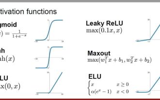 Analysis of commonly used AI activation functions: deep learning practice of Sigmoid, Tanh, ReLU and Softmax
Dec 28, 2023 pm 11:35 PM
Analysis of commonly used AI activation functions: deep learning practice of Sigmoid, Tanh, ReLU and Softmax
Dec 28, 2023 pm 11:35 PM
Activation functions play a crucial role in deep learning. They can introduce nonlinear characteristics into neural networks, allowing the network to better learn and simulate complex input-output relationships. The correct selection and use of activation functions has an important impact on the performance and training results of neural networks. This article will introduce four commonly used activation functions: Sigmoid, Tanh, ReLU and Softmax, starting from the introduction, usage scenarios, advantages, disadvantages and optimization solutions. Dimensions are discussed to provide you with a comprehensive understanding of activation functions. 1. Sigmoid function Introduction to SIgmoid function formula: The Sigmoid function is a commonly used nonlinear function that can map any real number to between 0 and 1. It is usually used to unify the
 Latent space embedding: explanation and demonstration
Jan 22, 2024 pm 05:30 PM
Latent space embedding: explanation and demonstration
Jan 22, 2024 pm 05:30 PM
Latent Space Embedding (LatentSpaceEmbedding) is the process of mapping high-dimensional data to low-dimensional space. In the field of machine learning and deep learning, latent space embedding is usually a neural network model that maps high-dimensional input data into a set of low-dimensional vector representations. This set of vectors is often called "latent vectors" or "latent encodings". The purpose of latent space embedding is to capture important features in the data and represent them into a more concise and understandable form. Through latent space embedding, we can perform operations such as visualizing, classifying, and clustering data in low-dimensional space to better understand and utilize the data. Latent space embedding has wide applications in many fields, such as image generation, feature extraction, dimensionality reduction, etc. Latent space embedding is the main
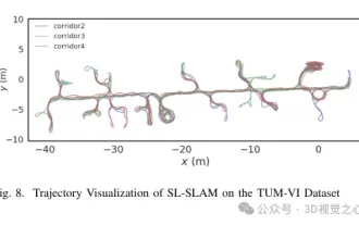 Beyond ORB-SLAM3! SL-SLAM: Low light, severe jitter and weak texture scenes are all handled
May 30, 2024 am 09:35 AM
Beyond ORB-SLAM3! SL-SLAM: Low light, severe jitter and weak texture scenes are all handled
May 30, 2024 am 09:35 AM
Written previously, today we discuss how deep learning technology can improve the performance of vision-based SLAM (simultaneous localization and mapping) in complex environments. By combining deep feature extraction and depth matching methods, here we introduce a versatile hybrid visual SLAM system designed to improve adaptation in challenging scenarios such as low-light conditions, dynamic lighting, weakly textured areas, and severe jitter. sex. Our system supports multiple modes, including extended monocular, stereo, monocular-inertial, and stereo-inertial configurations. In addition, it also analyzes how to combine visual SLAM with deep learning methods to inspire other research. Through extensive experiments on public datasets and self-sampled data, we demonstrate the superiority of SL-SLAM in terms of positioning accuracy and tracking robustness.
 From basics to practice, review the development history of Elasticsearch vector retrieval
Oct 23, 2023 pm 05:17 PM
From basics to practice, review the development history of Elasticsearch vector retrieval
Oct 23, 2023 pm 05:17 PM
1. Introduction Vector retrieval has become a core component of modern search and recommendation systems. It enables efficient query matching and recommendations by converting complex objects (such as text, images, or sounds) into numerical vectors and performing similarity searches in multidimensional spaces. From basics to practice, review the development history of Elasticsearch vector retrieval_elasticsearch As a popular open source search engine, Elasticsearch's development in vector retrieval has always attracted much attention. This article will review the development history of Elasticsearch vector retrieval, focusing on the characteristics and progress of each stage. Taking history as a guide, it is convenient for everyone to establish a full range of Elasticsearch vector retrieval.
 Understand in one article: the connections and differences between AI, machine learning and deep learning
Mar 02, 2024 am 11:19 AM
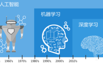
Understand in one article: the connections and differences between AI, machine learning and deep learning
Mar 02, 2024 am 11:19 AM
In today's wave of rapid technological changes, Artificial Intelligence (AI), Machine Learning (ML) and Deep Learning (DL) are like bright stars, leading the new wave of information technology. These three words frequently appear in various cutting-edge discussions and practical applications, but for many explorers who are new to this field, their specific meanings and their internal connections may still be shrouded in mystery. So let's take a look at this picture first. It can be seen that there is a close correlation and progressive relationship between deep learning, machine learning and artificial intelligence. Deep learning is a specific field of machine learning, and machine learning
 Super strong! Top 10 deep learning algorithms!
Mar 15, 2024 pm 03:46 PM
Super strong! Top 10 deep learning algorithms!
Mar 15, 2024 pm 03:46 PM
Almost 20 years have passed since the concept of deep learning was proposed in 2006. Deep learning, as a revolution in the field of artificial intelligence, has spawned many influential algorithms. So, what do you think are the top 10 algorithms for deep learning? The following are the top algorithms for deep learning in my opinion. They all occupy an important position in terms of innovation, application value and influence. 1. Deep neural network (DNN) background: Deep neural network (DNN), also called multi-layer perceptron, is the most common deep learning algorithm. When it was first invented, it was questioned due to the computing power bottleneck. Until recent years, computing power, The breakthrough came with the explosion of data. DNN is a neural network model that contains multiple hidden layers. In this model, each layer passes input to the next layer and
 AlphaFold 3 is launched, comprehensively predicting the interactions and structures of proteins and all living molecules, with far greater accuracy than ever before
Jul 16, 2024 am 12:08 AM
AlphaFold 3 is launched, comprehensively predicting the interactions and structures of proteins and all living molecules, with far greater accuracy than ever before
Jul 16, 2024 am 12:08 AM
Editor | Radish Skin Since the release of the powerful AlphaFold2 in 2021, scientists have been using protein structure prediction models to map various protein structures within cells, discover drugs, and draw a "cosmic map" of every known protein interaction. . Just now, Google DeepMind released the AlphaFold3 model, which can perform joint structure predictions for complexes including proteins, nucleic acids, small molecules, ions and modified residues. The accuracy of AlphaFold3 has been significantly improved compared to many dedicated tools in the past (protein-ligand interaction, protein-nucleic acid interaction, antibody-antigen prediction). This shows that within a single unified deep learning framework, it is possible to achieve
