

Knowledge of probability and statistics is at the core of data science and machine learning; we need knowledge of statistics and probability to effectively collect, review, and analyze data.
There are several real-world instances of phenomena that are considered statistical in nature (i.e. weather data, sales data, financial data, etc.). This means that in some cases we have been able to develop methods that help us simulate nature through mathematical functions that can describe the characteristics of the data. “A probability distribution is a mathematical function that gives the probability of occurrence of different possible outcomes in an experiment.” Understanding the distribution of data helps to better model the world around us. It can help us determine the likelihood of various outcomes, or estimate the variability of events. All of this makes understanding different probability distributions very valuable in data science and machine learning. Uniform distributionThe most direct distribution is uniform distribution. A uniform distribution is a probability distribution in which all outcomes are equally likely. For example, if we roll a fair die, the probability of landing on any number is 1/6. This is a discrete uniform distribution. But not all uniform distributions are discrete - they can also be continuous. They can take any real value within the specified range. The probability density function (PDF) of a continuous uniform distribution between a and b is as follows: Let's see how to encode them in Python:
import numpy as np
import matplotlib.pyplot as plt
from scipy import stats

# for continuous
a = 0
b = 50
size = 5000

X_continuous = np.linspace(a, b, size)
continuous_uniform = stats.uniform(loc=a, scale=b)
continuous_uniform_pdf = continuous_uniform.pdf(X_continuous)

# for discrete
X_discrete = np.arange(1, 7)
discrete_uniform = stats.randint(1, 7)
discrete_uniform_pmf = discrete_uniform.pmf(X_discrete)

# plot both tables
fig, ax = plt.subplots(nrows=1, ncols=2, figsize=(15,5))
# discrete plot
ax[0].bar(X_discrete, discrete_uniform_pmf)
ax[0].set_xlabel("X")
ax[0].set_ylabel("Probability")
ax[0].set_title("Discrete Uniform Distribution")
# continuous plot
ax[1].plot(X_continuous, continuous_uniform_pdf)
ax[1].set_xlabel("X")
ax[1].set_ylabel("Probability")
ax[1].set_title("Continuous Uniform Distribution")
plt.show()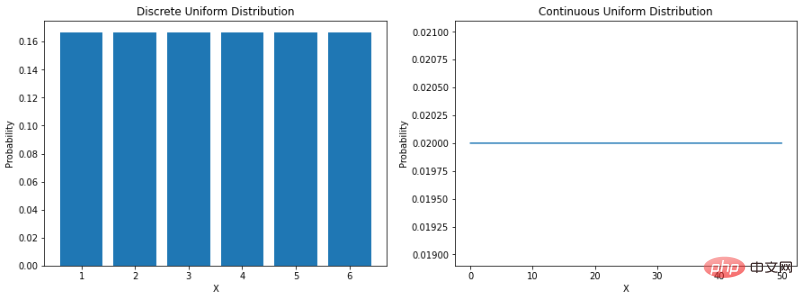
Gaussian distribution
The Gaussian distribution is probably the most commonly heard and familiar distribution. It has several names: some call it the bell curve because its probability plot looks like a bell, some call it the Gaussian distribution because the German mathematician Karl Gauss who first described it named it, and still others It's normally distributed because early statisticians noticed it happening over and over again. The probability density function of a normal distribution is as follows: σ is the standard deviation and μ is the mean of the distribution. Note that in a normal distribution, the mean, mode, and median are all equal. When we plot a normally distributed random variable, the curve is symmetrical about the mean—half the values are to the left of the center and half to the right of the center. And, the total area under the curve is 1.
mu = 0
variance = 1
sigma = np.sqrt(variance)
x = np.linspace(mu - 3*sigma, mu + 3*sigma, 100)

plt.subplots(figsize=(8, 5))
plt.plot(x, stats.norm.pdf(x, mu, sigma))
plt.title("Normal Distribution")
plt.show()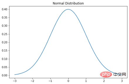
For normal distribution. The rule of thumb tells us what percentage of the data falls within a certain number of standard deviations from the mean. These percentages are:
The lognormal distribution is a continuous random variable with a lognormal distribution Probability distributions. Therefore, if the random variable X is lognormally distributed, then Y = ln(X) has a normal distribution. Here is the PDF of the lognormal distribution: A lognormally distributed random variable only takes on positive real values. Therefore, the lognormal distribution creates a right-skewed curve. Let’s plot it in Python:
X = np.linspace(0, 6, 500)

std = 1
mean = 0
lognorm_distribution = stats.lognorm([std], loc=mean)
lognorm_distribution_pdf = lognorm_distribution.pdf(X)

fig, ax = plt.subplots(figsize=(8, 5))
plt.plot(X, lognorm_distribution_pdf, label="μ=0, σ=1")
ax.set_xticks(np.arange(min(X), max(X)))

std = 0.5
mean = 0
lognorm_distribution = stats.lognorm([std], loc=mean)
lognorm_distribution_pdf = lognorm_distribution.pdf(X)
plt.plot(X, lognorm_distribution_pdf, label="μ=0, σ=0.5")

std = 1.5
mean = 1
lognorm_distribution = stats.lognorm([std], loc=mean)
lognorm_distribution_pdf = lognorm_distribution.pdf(X)
plt.plot(X, lognorm_distribution_pdf, label="μ=1, σ=1.5")

plt.title("Lognormal Distribution")
plt.legend()
plt.show()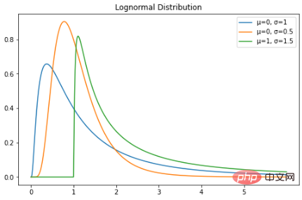
Poisson Distribution
The Poisson distribution is named after the French mathematician Simon Denis Poisson. This is a discrete probability distribution, which means that it counts events with finite outcomes - in other words, it is a counting distribution. Therefore, the Poisson distribution is used to show the number of times an event may occur within a specified period. If an event occurs at a fixed rate in time, then the probability of observing the number (n) of events in time can be described by a Poisson distribution. For example, customers may arrive at a coffee shop at an average rate of 3 times per minute. We can use the Poisson distribution to calculate the probability that 9 customers will arrive within 2 minutes. Here is the probability mass function formula: λ is the event rate in one unit of time – in our case, it is 3. k is the number of occurrences - in our case, it's 9. Scipy can be used here to complete the probability calculation.
from scipy import stats

print(stats.poisson.pmf(k=9, mu=3))
0.002700503931560479
The curve of the Poisson distribution is similar to the normal distribution, and λ represents the peak value.
X = stats.poisson.rvs(mu=3, size=500)

plt.subplots(figsize=(8, 5))
plt.hist(X, density=True, edgecolor="black")
plt.title("Poisson Distribution")
plt.show()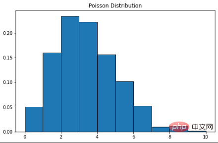
Exponential distribution
指数分布是泊松点过程中事件之间时间的概率分布。指数分布的概率密度函数如下:λ 是速率参数,x 是随机变量。
X = np.linspace(0, 5, 5000)

exponetial_distribtuion = stats.expon.pdf(X, loc=0, scale=1)

plt.subplots(figsize=(8,5))
plt.plot(X, exponetial_distribtuion)
plt.title("Exponential Distribution")
plt.show()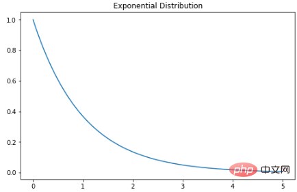
二项分布
可以将二项分布视为实验中成功或失败的概率。有些人也可能将其描述为抛硬币概率。参数为 n 和 p 的二项式分布是在 n 个独立实验序列中成功次数的离散概率分布,每个实验都问一个是 - 否问题,每个实验都有自己的布尔值结果:成功或失败。本质上,二项分布测量两个事件的概率。一个事件发生的概率为 p,另一事件发生的概率为 1-p。这是二项分布的公式:
可视化代码如下:
X = np.random.binomial(n=1, p=0.5, size=1000)

plt.subplots(figsize=(8, 5))
plt.hist(X)
plt.title("Binomial Distribution")
plt.show()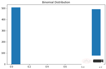
学生 t 分布
学生 t 分布(或简称 t 分布)是在样本量较小且总体标准差未知的情况下估计正态分布总体的均值时出现的连续概率分布族的任何成员。它是由英国统计学家威廉·西利·戈塞特(William Sealy Gosset)以笔名“student”开发的。PDF如下:n 是称为“自由度”的参数,有时可以看到它被称为“d.o.f.” 对于较高的 n 值,t 分布更接近正态分布。
import seaborn as sns
from scipy import stats

X1 = stats.t.rvs(df=1, size=4)
X2 = stats.t.rvs(df=3, size=4)
X3 = stats.t.rvs(df=9, size=4)

plt.subplots(figsize=(8,5))
sns.kdeplot(X1, label = "1 d.o.f")
sns.kdeplot(X2, label = "3 d.o.f")
sns.kdeplot(X3, label = "6 d.o.f")
plt.title("Student's t distribution")
plt.legend()
plt.show()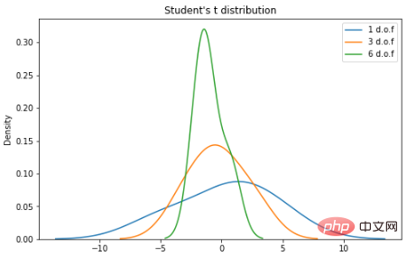
卡方分布
卡方分布是伽马分布的一个特例;对于 k 个自由度,卡方分布是一些独立的标准正态随机变量的 k 的平方和。PDF如下:这是一种流行的概率分布,常用于假设检验和置信区间的构建。在 Python 中绘制一些示例图:
X = np.arange(0, 6, 0.25)

plt.subplots(figsize=(8, 5))
plt.plot(X, stats.chi2.pdf(X, df=1), label="1 d.o.f")
plt.plot(X, stats.chi2.pdf(X, df=2), label="2 d.o.f")
plt.plot(X, stats.chi2.pdf(X, df=3), label="3 d.o.f")
plt.title("Chi-squared Distribution")
plt.legend()
plt.show()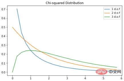
掌握统计学和概率对于数据科学至关重要。在本文展示了一些常见且常用的分布,希望对你有所帮助。
The above is the detailed content of Python implements eight probability distribution formulas and data visualization tutorials. For more information, please follow other related articles on the PHP Chinese website!


