
When we usually process data, we often find some duplicate data, which will not only reduce our work efficiency, but also affect our subsequent analysis of the data. Today I will share with you 4 ways to delete duplicate values in Excel without using formulas. Come and take a look!

In a table that records a lot of data, it is inevitable that there will be some duplicate records. If a field is unique and is not allowed to be repeated with other content, it is necessary to duplicate the records. Values are processed, and the common means are to delete duplicate data or modify the record content.
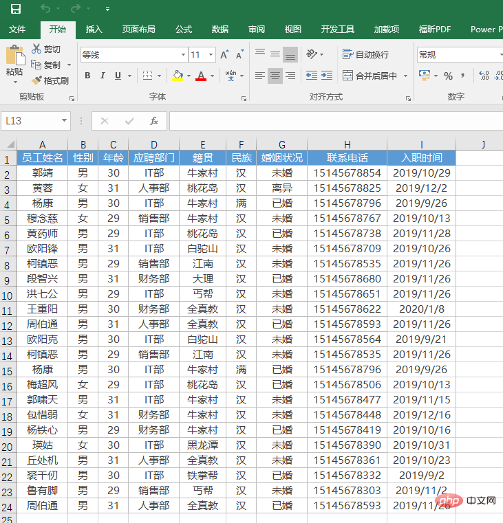
The following is an employee information statistics table. There are some duplicate items in it. How to find and delete duplicate items is the basis for table data processing.
Here are four ways to deal with repeated values of data without using formulas: ① Mark duplicates through conditional formatting; ② Delete duplicates through advanced filtering; ③ Delete duplicates directly through the "Remove Duplicates" function; ④ Delete duplicates through pivot tables.
Method 1: Mark duplicates through conditional formatting
Conditional formatting is a type of cell format, which can be known by its name. When the cell content meets a certain condition, a specified format is set for the cell. When the condition is not met, the original cell format remains unchanged.
If you only need to determine whether the unique data in a certain column in the table contains duplicate values, you can use conditional formatting to mark the duplicate values in the column, and then manually delete or modify the corresponding records. For example, in the above employee information statistics table, the employee name column contains duplicate values. We can select the employee name column and set conditional formatting to mark duplicates. The specific steps are as follows:
Select the unit to determine whether it has duplicate values. Cell area, click the "Conditional Formatting" button in the "Home" tab, select "Highlight Cell Rules", and click the "Duplicate Values" command to highlight the repeated data.
The limitation of this method is that conditional formatting can only filter single columns. If there are many columns, you need to filter column by column, which will increase a lot of workload. The following methods 2, 3, and 4 can avoid the above problems.
Method 2: Remove duplicates through advanced filtering
Filtering out qualified data is a routine operation in data management, which can Data that does not meet the conditions are temporarily hidden, and you can accurately find the data you need. Advanced filtering can filter the data in the target area based on multiple conditions within an area, and you can also set the display location of the filtered results. The specific steps are as follows:
Select any cell in the original data area, click the "Advanced" button in the "Data" tab, and start the advanced filtering function.
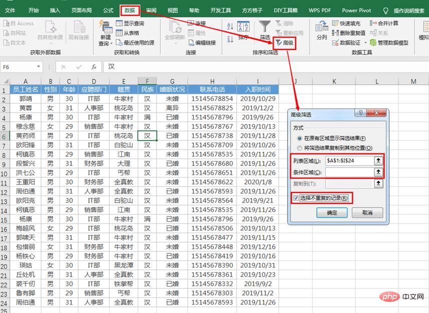
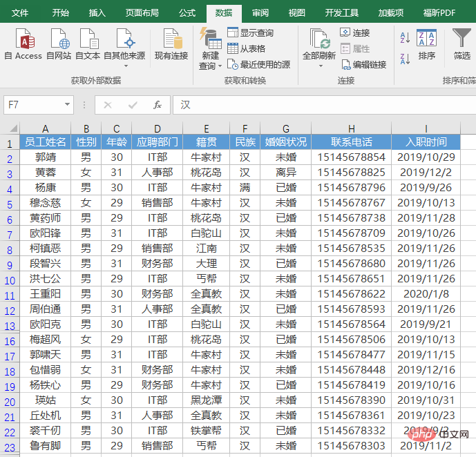
Advanced filtering will automatically identify a continuous data area and fill it in the "list area". (Note: There is no need to fill in the "condition area" here) Check the "Select non-duplicate records" check box and click the "OK" button to display non-duplicate items.
Method 3: Directly delete duplicate items through the "Delete Duplicate Values" function
EXCEL provides The function of directly deleting duplicate items can determine whether the data is duplicated based on the columns specified by the user, and delete the data deemed to be duplicated. The specific steps are as follows:
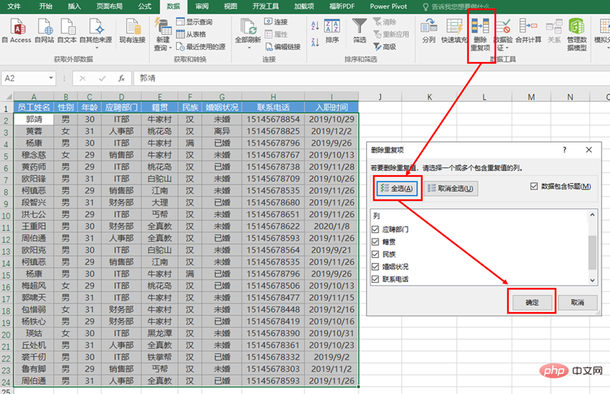
Select any cell in the data area, click the "Delete Duplicates" button in the "Data Tools" group under the "Data" tab, and click the "Delete Duplicates" button that opens In the dialog box, set the columns to be compared, and then click the "OK" button. Excel will determine whether there are duplicates in the table based on the specified column area, and automatically delete the found duplicates.
The effect is as shown in the figure below:

When setting the comparison column to delete duplicates, you should usually all Select all columns so that completely duplicate records can be compared. If you select only one column or select fewer columns, some data may be deleted by mistake. For example, when deleting duplicate items in an employee information statistics table, you cannot only use employee names as comparison conditions, otherwise some employee data with the same name and surname will be deleted. Generally, the unselected comparison columns are mostly sequence data that have no practical meaning, or data that is irrelevant to whether they are repeated or not.
Method 4: Remove duplicates through PivotTable
A PivotTable is a summary report generated from the database through which data can be dynamically changed The layout allows you to analyze data in different ways, and you can quickly combine and compare data to make it easier to analyze and process the data. It can be said that pivot tables are the most powerful function in Excel, bar none. The following introduces the function of deleting duplicates in pivot tables, which is very practical. The specific steps are as follows:
① Select the cell range, click the "PivotTable" button in the "Insert" tab, select "Existing Worksheet", and select a blank space of the workbook in "Position" area, click OK.
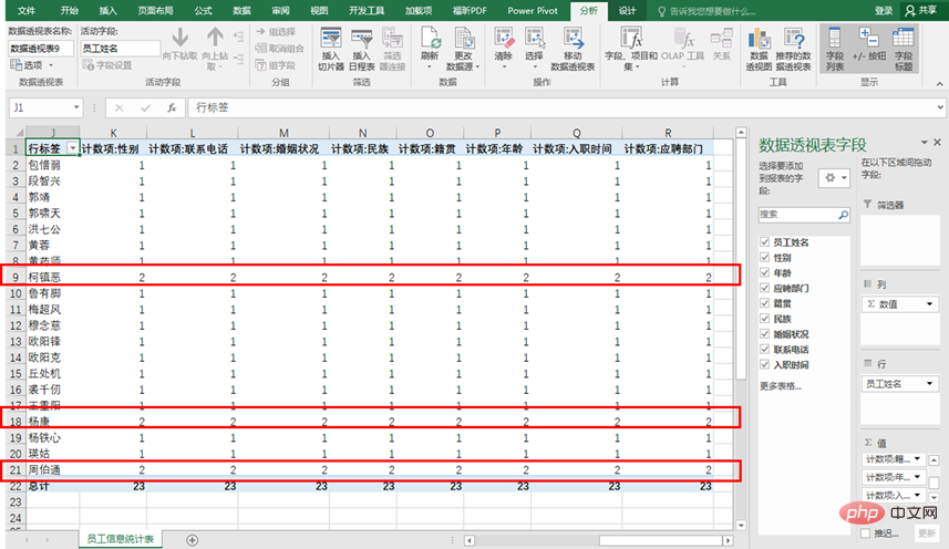
② In the pivot table field, drag "Employee Name" into the "Row" field, and change "Gender", "Age", "Applying Department", " Drag "Place of Place", "Ethnicity", "Marital Status", "Contact Number", and "Joining Time" into the "Value" field. And set the value aggregation method of "Age" and "Contact Number" to "Count".
#The effect is as follows, where rows with count items other than 1 represent duplicates.
Today’s content ends here. Do you guys know any other ways to deal with duplicate values? Leave a message in the comment area and tell us!
Related learning recommendations: excel tutorial
The above is the detailed content of Sharing practical Excel skills: 4 tips for deleting duplicate values!. For more information, please follow other related articles on the PHP Chinese website!
 Compare the similarities and differences between two columns of data in excel
 excel duplicate item filter color
 How to copy an Excel table to make it the same size as the original
 Excel table slash divided into two
 Excel diagonal header is divided into two
 Absolute reference input method
 java export excel
 Excel input value is illegal


![[Web front-end] Node.js quick start](https://img.php.cn/upload/course/000/000/067/662b5d34ba7c0227.png)


