
You may be a data collector in an organization or in a school or college. You may have an excel file that may need to be filled in by many different people. The way people enter data is up to them and may contain many errors or even data that may not be within the required range. At the end of the day, you're probably going to have a huge headache correcting and replacing all the data in the world.
So, is there a way to limit the data that can be entered into a specific cell, such as forcing a dropdown? When you force a drop-down menu for a specific cell, data can only be entered into that cell if it is within the drop-down range.
In this article, we explain how to easily add a drop-down menu to an Excel cell in some simple steps. Hope you found this article useful.
Step 1: Next to the Windows Start menu icon, click the Search icon on the taskbar .

Step 2: In the search bar window, search for Microsoft excel and click from the Best Match section Click Excel.

Step 3: Once excel starts, we will first create the drop down menu content. In this example, we will create it on Sheet2 in Excel. To do this, click Sheet2 at the bottom of the Excel window, as shown in the screenshot below.

Step 4: Now in Sheet2, enter the drop-down menu content at any position. I have used column A to enter my content.
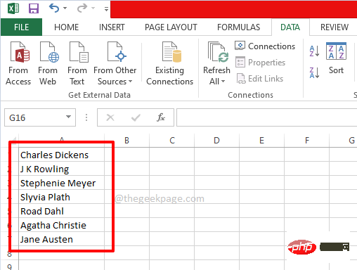
Step 5: Once the dropdown menu source is ready, let’s use the source content in the main Excel sheet.
To do this, click Sheet1 at the bottom of the window and select all the cells to which you want the drop-down menu to apply. Alternatively, if you wish to apply the drop-down menu to a single cell, just click on that single cell.
In the example below, I have a column called Author and I have selected some cells from A2 to A13 and I want to apply the dropdown menu to these cells each in the grid.
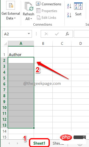
Step 6: Again, make sure your cell is selected. You can even select individual cells, which is really nice.
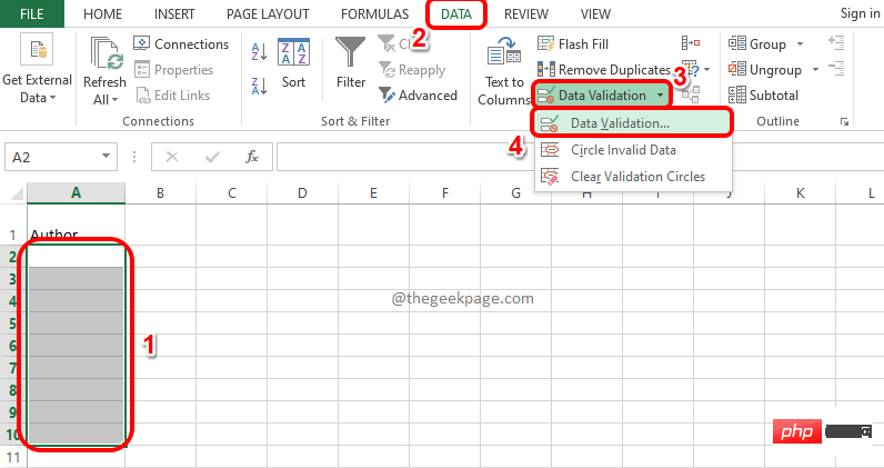
Next, click on the DATA tab on the top panel. Now, click on the Data Validation drop-down menu and click on the Data Validation option.
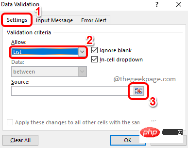
Step 7: You will now have the Data Validation window open in front of you. First click on the "Settings" tab. Now, from the drop-down menu associated with the option Allow, click on the option named List. Finally, click on the Source icon to select a source list.
If you have any questions, please see the screenshot below.
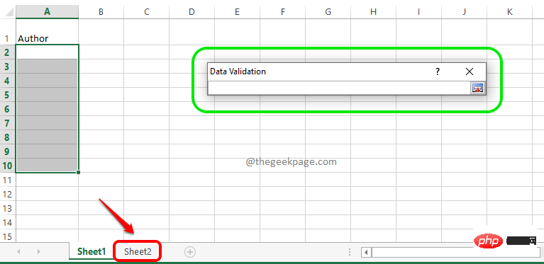
Step 8: You will be able to see the Data Validation window (marked green), now in this window No action is required.
Since the drop-down menu source is in Sheet2, click Sheet2 first.
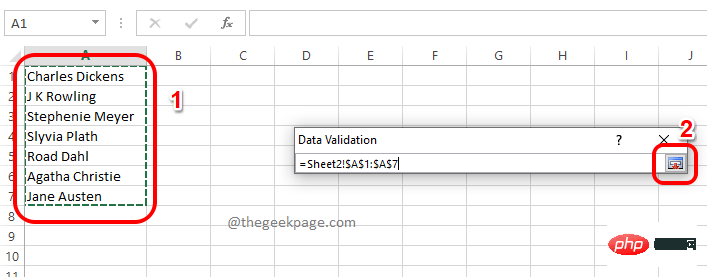
Step 9: Now just drag and select the cells you prepared earlier. Once you select a source cell, the data validation window will automatically populate. Finally, click the Source icon again.
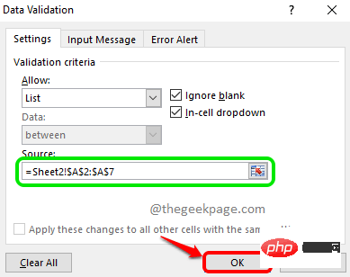
Step 10: Once you return to the data validation window, you will be able to see that the source list is populated. Just click the OK button.
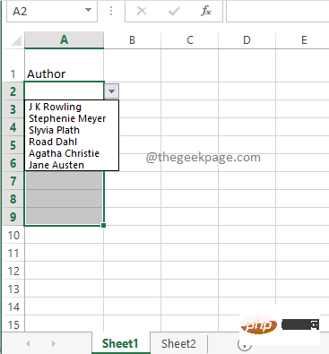
Step 11: You will now return to the main worksheet, Sheet1. Viola, you can now see that all of the cells you originally selected now have the dropdown menu applied to them.
Only the value from the drop-down source menu can be assigned to each of these cells. enjoy!
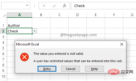
If you try to double-click a cell and then try to enter a value that does not exist in the drop-down source, you will receive a message that you entered Invalid value . In this way, the purpose of limiting the values that can be entered into the cell is achieved.
The above is the detailed content of How to add a drop-down menu in Microsoft Excel. For more information, please follow other related articles on the PHP Chinese website!
 Cell sum
 js gets current time
 What does pycharm mean when running in parallel?
 css3transition
 Introduction to the main work content of front-end engineers
 How to connect php to mssql database
 The difference between Hongmeng system and Android system
 How to open the download permission of Douyin
 tim mobile online


