

How to fix formula parsing errors in Google Sheets

What are formula parsing errors in Google Sheets?
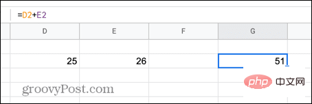
Formula parsing errors occur in Google Sheets when the application cannot handle the instructions in the formula. This is usually because there's a problem with the formula itself, or there's a problem with the cells the formula refers to.
There are many different types of formula parsing errors in Google Sheets. How to fix formula parsing errors in Google Sheets depends on the type of error your formula produces.
We'll look at some of the most common formula parsing errors below and how to fix them.
How to fix #ERROR! Error
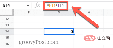
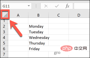
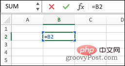
#Error in Google Sheets! Formula parsing errors occur when Google Sheets doesn't understand your formula but isn't sure what the problem is. When you see a formula parsing error in your spreadsheet, you can view more information about the error by hovering your mouse over the small red triangle in the upper-right corner of the cell. 
For many of the errors below, this will provide some useful information about the cause of the error. In case of #ERROR! Formula parsing error, this box does not provide any information that we do not know. 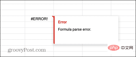
Unfortunately, #ERROR! is one of the most difficult formula parsing errors to fix. You'll be stuck with nothing to do, and the reason could be one of many different problems.
If your formula is complex, find out the cause of the #ERROR! Information can be challenging - but not impossible.
FIX #ERROR! Message in Google Sheets:
- Click on the cell containing the formula.
- Check if you are missing any operators via the formula. For example, missing numbers may cause this error.
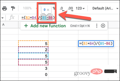
- Check whether the number of open brackets matches the number of closing brackets.
- Check that your cell references are correct. For example, a formula that uses A1 A5 instead of A1:A5 will produce this error.
- See if you include the $ symbol anywhere in the formula to reference currency. This symbol is used for absolute references to cells, so it can cause this error if used incorrectly.
- If you still can't find the source of the error, try recreating your formula from scratch. When you start entering any formula in Google Sheets, use the helper that appears to make sure your formula has the correct syntax.
How to Fix #N/A Error in Google Sheets
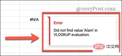
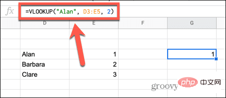
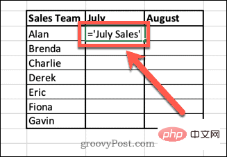
Occurs when the value or string you are looking for is not found in the given range# N/A error. This may be because you are looking for a value that is not in the list, or because you entered the wrong search key.
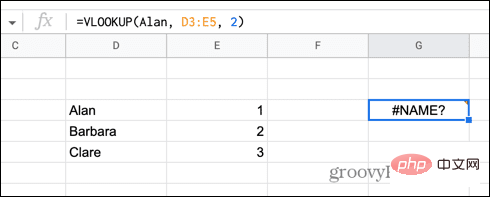
This error is usually found when using functions such as VLOOKUP and HLOOKUP. The good news is that hovering your mouse over the red triangle will usually give you some useful information on how to fix the problem.
To fix #N/A errors in Google Sheets:
- Hover your mouse over the red triangle in the cell showing the error.

- You should see some information about the cause of the error.
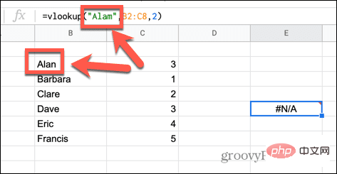
- In this example, the formula is searching for the name "Alam", but the correct spelling of the name in the list is "Alan".
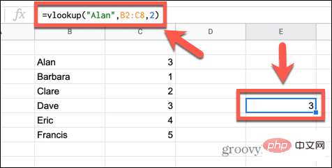
- Correct the spelling in the formula and the error disappears.
- Other possible causes of the error may be that your data does not contain the search key you are looking for, or that you entered the wrong range. Recheck your formula to make sure each part is correct and your errors should be fixed.

How to fix #DIV/0! Error in Google Sheets
This error is common when you use formulas that involve mathematical division. The error indicates that you are trying to divide by zero. This is a calculation that Google Sheets cannot perform because mathematically the answer is undefined.
Fix #DIV/0! Error in Google Sheets:
- Click on the cell containing the error.
- Look for the division sign ( / ) in the formula.
- Highlight the part to the right of the symbol and you should see a value pop up above the highlighted area. If this value is zero, your highlighted section is #DIV/0!
- # Repeat this for any other part of the formula.
- When you find all instances of division by zero, changing or removing these parts should eliminate the error.
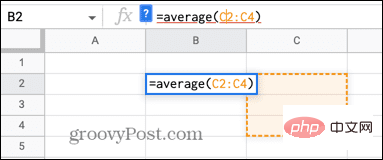
- You may also get this error when using functions that use division in their calculations (such as AVERAGE).
- This usually means that the range you selected contains no values.
- Changing your scope should fix this.
How to fix #REF! Error
#REF in Google Sheets! Error means you have an invalid cell reference in your formula. This could be because you are referring to a cell that does not exist, because you are referring to a cell outside the selected range, or because you have a circular reference. Hovering over the red triangle will tell you what issue caused your error.
Reference does not exist #REF! Error
When you hover over an error cell, you may see a reference not existing message. 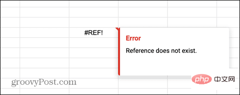
If you see this error, it means that at least one of the cells referenced in your formula no longer exists. This usually happens if you delete the row or column that contains the cells referenced in the formula.
Fix non-existent reference #REF! Error:
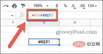
- Click the cell that contains the error.
- Looking for#REF! Within the formula itself.
- Replace this part of the formula with a value or a valid cell reference.
- The error will now disappear.
Out of range #REF! Error
If you hover over a cell that contains an error, you may see a message stating that the formula evaluated out of range. 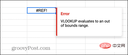
This means that your formula refers to cells that are not included in the range you specified.
Fix out of bounds range #REF! Error:
- Click the cell that contains the error.
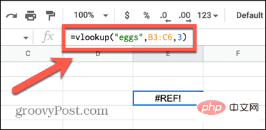
- Check the formula in that cell for any references to cells outside the range.
- In this example, the range references the values in columns B and C, but requires the formula to return a value from the third column in the range. Since the range only contains two columns, the third column is outside the range.
- Either increase the range to include three columns or change the index to 1 or 2 and the error will go away.
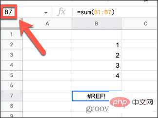
Circular dependency #REF! Error
Hover over #REF! Error cells may show that the problem is due to a circular dependency. 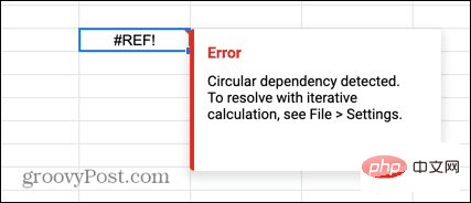
This means the formula is trying to reference itself. This is a common mistake when you try to find the sum of a column of numbers and you may accidentally include cells in the range that contain your formula.
Fix circular dependencies #REF! mistake:
- Click on the cell containing the error.
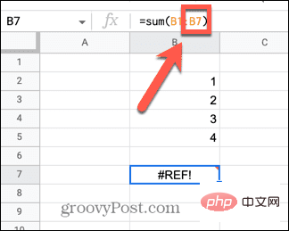
- Write down the reference to this cell, such as B7.
- Look for this cell reference in your formula. The cell may not appear explicitly in your formula; it may be included in a range.
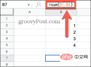
- Remove any reference to the cell containing the formula from the formula itself and the error will go away.
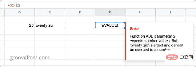
How to fix #VALUE! Error
# value in Google Sheets! The error occurs when you use a formula that requires a numeric value but uses or references a cell that contains a text string. Hovering the mouse over a cell can provide very useful information about the exact cause of the problem.
FIX #VALUE! Errors in Google Sheets:
- Hover your mouse over the cell containing the error.
- You will see information about which part of the formula caused the error. If your cells contain any spaces, these may cause the cell to be treated as text rather than a value.
- Replace the offending part of the formula with the value or a reference to the value and the error will disappear.
How to fix #NAME? Error
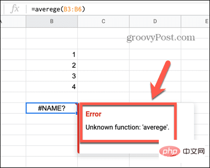
#NAME in Google Sheets? error means you entered a spelling error in the formula, or you omitted or used the wrong quotation marks. Hovering your mouse over a cell can help you determine which part of the formula is incorrect.
FIX #NAME? Errors in Google Sheets:
- Hover over the error cell.
- You will see information about which part of the formula is unrecognized.
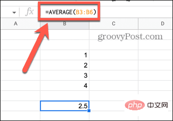
- If the word is obviously misspelled, correct the spelling and the mistake should go away.
- If the word is spelled correctly, find the part of the formula that contains the word.
- Try adding or removing quotes around the word and the error message may disappear.
How to fix #NUM! Error
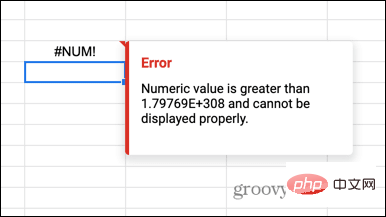
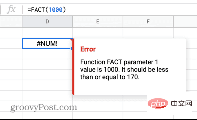
#NUM in Google Sheets! This error means that you are trying to calculate a value that is larger than Google Sheets can calculate or display. Hovering the mouse over a cell provides information about the cause.
Fix #NUM! Errors in Google Sheets:
- Hover your mouse over the cell containing the error.
- If the result of a formula is too large to be displayed, you will see an associated error message. Reduce the size of the value to fix the error.
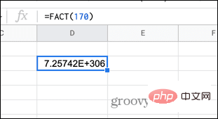
- If the result of a formula is too large to be calculated, hovering over the cell may give you the maximum value you can use in the formula.
- Staying within this range will fix the error.
The above is the detailed content of How to fix formula parsing errors in Google Sheets. For more information, please follow other related articles on the PHP Chinese website!

Hot AI Tools

Undresser.AI Undress
AI-powered app for creating realistic nude photos

AI Clothes Remover
Online AI tool for removing clothes from photos.

Undress AI Tool
Undress images for free

Clothoff.io
AI clothes remover

AI Hentai Generator
Generate AI Hentai for free.

Hot Article
Hot Tools

Notepad++7.3.1
Easy-to-use and free code editor

SublimeText3 Chinese version
Chinese version, very easy to use

Zend Studio 13.0.1
Powerful PHP integrated development environment

Dreamweaver CS6
Visual web development tools

SublimeText3 Mac version
God-level code editing software (SublimeText3)
Hot Topics
 1371
1371
 52
52

 How to fix formula parsing errors in Google Sheets
May 05, 2023 am 11:52 AM
How to fix formula parsing errors in Google Sheets
May 05, 2023 am 11:52 AM
What are formula parsing errors in Google Sheets? Formula parsing errors occur in Google Sheets when the application cannot handle the instructions in the formula. This is usually because there's a problem with the formula itself, or there's a problem with the cells the formula refers to. There are many different types of formula parsing errors in Google Sheets. The method for fixing formula parsing errors in Google Sheets depends on the type of error your formula produces. We'll look at some of the most common formula parsing errors below and how to fix them. How to fix #ERROR! Error in Google Sheets #Error! Formula parsing errors occur when Google Sheets doesn't understand your formula but isn't sure what the problem is. When you are on the spreadsheet
 How to find and delete merged cells in Excel
Apr 20, 2023 pm 11:52 PM
How to find and delete merged cells in Excel
Apr 20, 2023 pm 11:52 PM
How to Find Merged Cells in Excel on Windows Before you can delete merged cells from your data, you need to find them all. It's easy to do this using Excel's Find and Replace tool. Find merged cells in Excel: Highlight the cells where you want to find merged cells. To select all cells, click in an empty space in the upper left corner of the spreadsheet or press Ctrl+A. Click the Home tab. Click the Find and Select icon. Select Find. Click the Options button. At the end of the FindWhat settings, click Format. Under the Alignment tab, click Merge Cells. It should contain a check mark rather than a line. Click OK to confirm the format
 How to create a custom power plan on Windows 11
Apr 28, 2023 am 11:34 AM
How to create a custom power plan on Windows 11
Apr 28, 2023 am 11:34 AM
How to Create a Custom Power Plan on Windows 11 Custom power plans allow you to determine how Windows reacts to different situations. For example, if you want your monitor to turn off after a certain amount of time, but don't want it to go to sleep, you can create a custom schedule to do this. Create a custom power plan on Windows 11: Open the Start menu and type control panel. Select Control Panel from the search results. In Control Panel, change the View by option to Large icons. Next, select Power Options. Click the Create power plan option in the Power Options menu. Select the basic power plan you want to use from the options provided. Give it a descriptive name in the Plan Name field at the bottom
 How to calculate the difference between dates on Google Sheets
Apr 19, 2023 pm 08:07 PM
How to calculate the difference between dates on Google Sheets
Apr 19, 2023 pm 08:07 PM
If you are tasked with working with a spreadsheet containing a large number of dates, calculating the difference between multiple dates can be very frustrating. While the easiest option is to rely on an online date calculator, it may not be the most convenient as you may have to enter the dates one by one into the online tool and then manually copy the results into a spreadsheet. For large numbers of dates, you need a tool that gets the job done more conveniently. Fortunately, Google Sheets allows users to locally calculate the difference between two dates in a spreadsheet. In this post, we will help you calculate the number of days between two dates on Google Sheets using some built-in functions. How to calculate the difference between dates on Google Sheets if you want Google
 How to sum columns in Excel
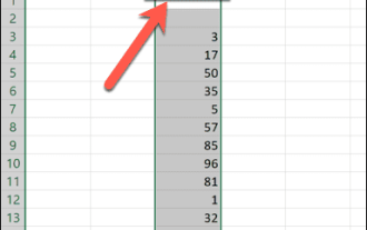
May 16, 2023 pm 03:26 PM
How to sum columns in Excel
May 16, 2023 pm 03:26 PM
How to Quickly View the Total of a Column in Excel If you just want to know the total of a column without adding that information to your spreadsheet, you can use the Excel status bar to quickly view the total of a column or any range of cells. To see the sum of a column using the Excel status bar: Highlight the data you want to summarize. To select an entire column, click the column name. Otherwise, drag cells to select your range. At the bottom of the screen, you'll see information about your selection, such as the average of all values and the number of data points in the range. You will also see the sum of all values in the selected cells. How to sum columns in Excel using AutoSum If you wish to add the sum of a column to a spreadsheet, there are many situations
 How to remove time from date in Excel
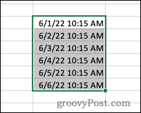
May 17, 2023 am 11:22 AM
How to remove time from date in Excel
May 17, 2023 am 11:22 AM
Change Date Format in Excel Using Number Format The easiest way to remove time from a date in Excel is to change the number format. This does not remove the time from the timestamp - it just prevents it from displaying in your cell. If you use these cells in calculations, the time and date are still included. To change the date format in Excel using number format: Open your Excel spreadsheet. Select the cell containing your timestamp. In the main menu, select the down arrow at the end of the number format box. Choose a date format. After changing the format, the time will stop appearing in your cells. If you click on one of the cells, the time format is still visible in the formula bar. Use cell formatting
 How to find circular references in Excel?
May 08, 2023 pm 04:58 PM
How to find circular references in Excel?
May 08, 2023 pm 04:58 PM
What are circular references in Excel? As the name suggests, a circular reference in Excel is a formula that refers to the cell where the formula is located. For example, a formula can directly reference the cell in which the formula resides: The formula can also refer to itself indirectly by referencing other cells, which in turn refer to the cell in which the formula resides: In most cases, circular references are not needed and are created incorrectly; formulas that reference themselves typically do not provide any useful functionality. There are some situations where you might want to use a circular reference, but in general if you create a circular reference it's probably a bug. How to Find Circular References in Excel Excel can help you by giving you a warning the first time you try to create a circular reference.
 How to extract data from another worksheet in Excel?
Apr 23, 2023 pm 03:43 PM
How to extract data from another worksheet in Excel?
Apr 23, 2023 pm 03:43 PM
How to use cell references to pull data from another worksheet in Excel You can use related cell references to pull data from one Excel worksheet to another. This is a simple way to get data from one worksheet to another. To extract data from another worksheet using cell references in Excel: Click on the cell where you want to display the extracted data. Type = (equal sign) followed by the name of the worksheet from which you want to extract data. If the worksheet name is longer than one word, enclose the worksheet name in single quotes. Enter! followed by the cell reference of the cell to be pulled. Press Enter. Values from other worksheets will now appear in the cells. If you want to pull more values,