 Technology peripherals
 AI
AI
 Comparison summary of five deep learning models for time series forecasting
Comparison summary of five deep learning models for time series forecasting
The Makridakis M-Competitions series (called M4 and M5 respectively) were held in 2018 and 2020 respectively (M6 was also held this year). For those who don’t know, the m-series can be thought of as a summary of the current state of the time series ecosystem, providing empirical and objective evidence for current theory and practice of forecasting.
The results of the 2018 M4 showed that pure “ML” methods outperformed traditional statistical methods by a large extent that was unexpected at the time. In M5[1] two years later, the highest score was with only "ML" methods. And all the top 50 are basically ML based (mostly tree models). This competition saw the debut of LightGBM (for time series forecasting) as well as Amazon's Deepar [2] and N-Beats [3]. The N-Beats model was released in 2020 and is 3% better than the M4 competition winner!
The recent Ventilator Pressure Prediction competition demonstrated the importance of using deep learning methods to tackle real-time time series challenges. The goal of the competition is to predict the temporal sequence of pressures within a mechanical lung. Each training instance is its own time series, so the task is a multiple time series problem. The winning team submitted a multi-layer deep architecture that included an LSTM network and a Transformer block.
In the past few years, many famous architectures have been released, such as MQRNN and DSSM. All these models contribute many new things to the field of time series forecasting using deep learning. In addition to winning Kaggle competitions, it also brought us more progress such as:
- Versatility: the ability to use the model for different tasks.
- MLOP: The ability to use models in production.
- Interpretability and Interpretability: Black box models are not that popular.
This article discusses 5 deep learning architectures that specialize in time series prediction. The paper is:
- N-BEATS(ElementAI)
- DeepAR (Amazon)
- Spacetimeformer[4]
- Temporal Fusion Transformer or TFT(Google) [5]
- TSFormer (MAE in time series)[7]
N-BEATS
This model comes directly from the (unfortunately) short-lived ElementAI company, which was co-founded by Yoshua Bengio. The top-level architecture and its main components are shown in Figure 1:
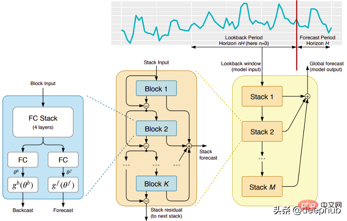
N-BEATS is a pure deep learning architecture based on integrating deep stacks of feedforward networks that Stacking is also done via forward and reverse interconnections.
Each block only models the residual error produced by the previous backcast, and then updates the prediction based on this error. This process simulates the Box-Jenkins method when fitting an ARIMA model.
The following are the main advantages of this model:
Expressive and easy to use: The model is easy to understand, has a modular structure, it is designed to require minimal time series feature engineering and does not require The input needs to be scaled.
The model has the ability to generalize across multiple time series. In other words, different time series with slightly different distributions can be used as input. In N-BEATS, it is implemented through meta-learning. The meta-learning process includes two processes: internal learning process and external learning process. The internal learning process occurs inside the block and helps the model capture local temporal features. The external learning process occurs in stacking layers and helps the model learn global features of all time series.
Double residual stacking: The idea of residual connection and stacking is very clever, and it is used in almost every type of deep neural network. The same principle is applied in the implementation of N-BEATS, but with some additional modifications: each block has two residual branches, one running in the lookback window (called backcast) and the other running in the prediction window (called for forecast).
Each consecutive block models only the residual resulting from the reconstructed backcast of the previous block, and then updates the prediction based on that error. This helps the model better approximate the useful backcast signal, while the final stack prediction prediction is modeled as a hierarchical sum of all partial predictions. It is this process that simulates the Box-Jenkins method of the ARIMA model.
Interpretability: The model comes in two variants, general and interpretable. In the general variant, the network arbitrarily learns the final weights of the fully connected layers of each block. In the interpretable variant, the last layer of each block is removed. The backcast and forecast branches are then multiplied by specific matrices simulating trend (monotonic function) and seasonality (cyclical cyclic function).
Note: The original N-BEATS implementation only works with univariate time series.
DeepAR
A novel time series model that combines deep learning and autoregressive features. Figure 2 shows the top-level architecture of DeepAR:

Here are the main advantages of this model:
DeepAR works very well on multiple time series: by using multiple time series with slightly different distributions. Build a global model. Also applicable to many real-life scenarios. For example, a power company may want to launch a power forecasting service for each customer, each of which has different consumption patterns (which means different distributions).
In addition to historical data, DeepAR also allows the use of known future time series (a characteristic of autoregressive models) and additional static attributes. In the electricity demand forecasting scenario mentioned earlier, an additional time variable could be the month (as an integer with a value between 1-12). Assuming each customer is associated with a sensor that measures power consumption, the additional static variables would be something like sensor_id or customer_id.
If you are familiar with using neural network architectures such as MLPs and RNNs for time series forecasting, a key preprocessing step is to scale the time series using normalization or normalization techniques. This does not require manual operation in DeepAR, because the underlying model scales the autoregressive input z for each time series i by a scaling factor v_i, which is the mean of that time series. Specifically, the scale factor equation used in the paper benchmark is as follows:

#But in practice, if the size of the target time series varies greatly, then during the preprocessing It is still necessary to apply your own scaling. For example, in an energy demand forecasting scenario, the data set may contain medium-voltage electricity customers (such as small factories, consuming electricity in megawatt units) and low-voltage customers (such as households, consuming electricity in kilowatt units).
DeepAR makes probability predictions instead of directly outputting future values. This is done as a Monte Carlo sample. These predictions are used to compute quantile predictions by using the quantile loss function. For those unfamiliar with this type of loss, quantile loss is used to compute not just an estimate, but a prediction interval around that value.
Spacetimeformer
Time dependence is the most important in univariate time series. But in multiple time series scenarios, things are not that simple. For example, suppose we have a weather forecast task and want to predict the temperature of five cities. Let's assume these cities belong to a country. Given what we have seen so far, we can use DeepAR and model each city as an external static covariate.
In other words, the model will consider both temporal and spatial relationships. This is the core idea of Spacetimeformer: use a model to exploit the spatial relationships between these cities/places, thereby learning additional useful dependencies, since the model will take into account both temporal and spatial relationships.
In-depth study of space-time sequences
As the name suggests, this model uses a structure based on transformers internally. When using transformers-based models for time series prediction, a popular technique for producing time-aware embeddings is to pass the input through a Time2Vec [6] embedding layer (for NLP tasks, positional encoding vectors are used instead of Time2Vec). While this technique works great for univariate time series, it doesn't make sense for multivariate time inputs. It may be that in language modeling, each word in a sentence is represented by an embedding, and a word is essentially a part of the vocabulary, while time series is not that simple.
In multivariate time series, at a given time step t, the input form is x_1,t, x2,t, x_m,t where x_i,t is the value of feature i, m is the feature/ The total number of sequences. If we pass the input through a Time2Vec layer, a temporal embedding vector will be produced. What does this embedding really represent? The answer is that it will represent the entire input collection as a single entity (token). So the model will only learn the temporal dynamics between time steps but will miss the spatial relationships between features/variables.
Spacetimeformer solves this problem by flattening the input into a large vector called a spacetime sequence. If the input contains N variables, organized into T time steps, the resulting spatiotemporal sequence will have the (NxT) label. Figure 3 below shows this better:
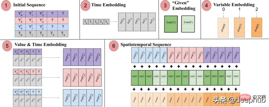
The paper states: "(1) Multivariate input format containing time information. The decoder input is missing ("?") values and is set to zero when making predictions. (2) The time series is passed through a Time2Vec layer, generating a representative Frequency embedding of periodic input patterns. (3) Binary embedding indicates whether the value is given as context or needs to be predicted. (4) Map the integer index of each time series to a "spatial" representation with a lookup table embedding . (5) Utilize a feed-forward layer to project the Time2Vec embedding and variable values of each time series. (6) Summing values and time, variables and a given embedding results in making the MSA more consistent between time and variable space. A long sequence is taken as input.
In other words, the final sequence encodes a unified embedding that contains temporal, spatial and contextual information. But a disadvantage of this method is that the sequence may become very long Resulting in a quadratic growth of resources. This is because according to the attention mechanism, each token is checked against another. The authors use a more efficient architecture called the Performer attention mechanism, which is suitable for larger sequences.
Temporal Fusion Transformer
Temporal Fusion Transformer (TFT) is a Transformer-based time series prediction model released by Google. TFT is more versatile than previous models.
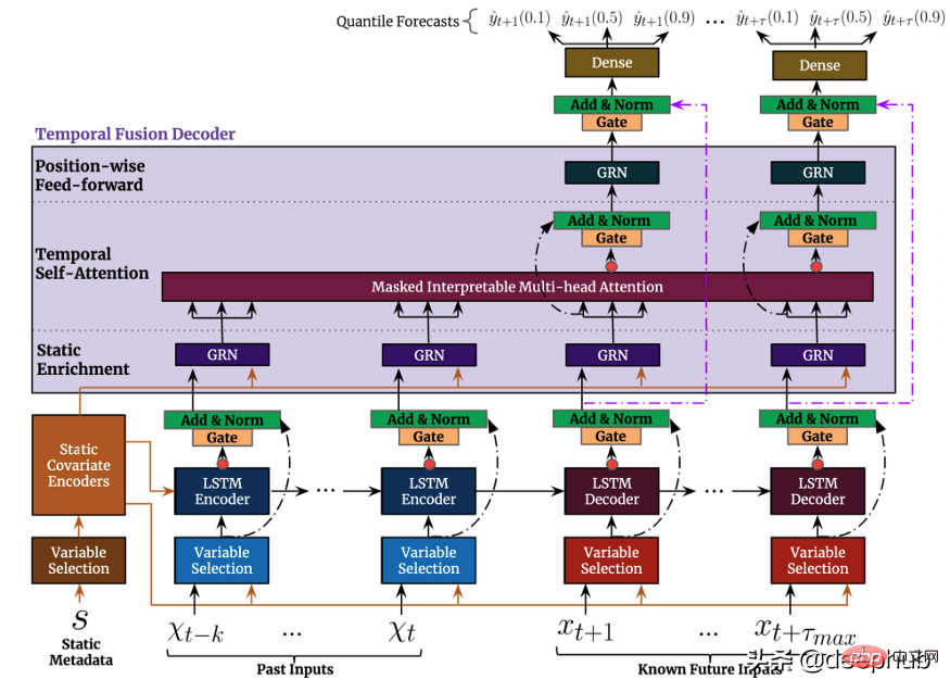
The top-level architecture of TFT is shown in Figure 4. The following are the main advantages of this model:
Like the previously mentioned model, TFT supports building on multiple heterogeneous time series Model.
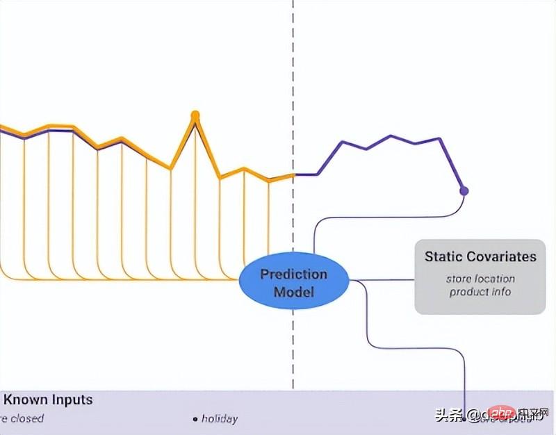
TFT supports three types of features: i) Time-varying data with known future inputs ii) Time-varying data known only so far iii) Categorical/static variables, also known as is a time-invariant feature. Therefore TFT is more versatile than previous models. In the power demand forecasting scenario mentioned earlier, we want to use humidity level as a time-varying feature, which was not known until now. This is in TFT is feasible, but not in DeepAR.
Figure 5 shows an example of how to use all these features:
TFT places a strong emphasis on interpretability. Specifically, by leveraging the Variable Selection component (shown in Figure 4 above), the model can successfully measure the impact of each feature. Therefore, it can be said that the model learns the importance of features.
On the other hand, TFT A new interpretable multi-head attention mechanism is proposed: the attention weights of this layer can reveal which time steps are most important during the lookback period. Visualization of these weights can reveal the most significant seasonal patterns in the entire dataset.
Prediction intervals: Similar to DeepAR, TFT outputs prediction intervals and predicted values by using quantile regression.
In summary, deep learning has undoubtedly revolutionized the landscape of time series forecasting. In addition to their unparalleled performance, all of the above models have one thing in common: they make full use of multiple, multivariate temporal data, and they use exogenous information to improve predictive performance to unprecedented levels. However, most of the natural language processing (NLP) tasks utilize pre-trained models. The feed of NLP tasks is mostly data created by humans. It is full of rich and excellent information and can almost be regarded as a data unit. In time series forecasting, we can feel the lack of such pre-trained models. Why can't we take advantage of this in time series like we do in NLP?
This leads to the last model we want to introduce, TSFormer. This model considers two perspectives. We divide it into four parts from input to output, and provides Python implementation code (officially also provided ), this model was just released, so we focus on it here.
TSFormer
It is an unsupervised time series pre-training model based on Transformer (TSFormer), which uses the training strategy in MAE and is able to capture very long dependencies in the data.
NLP and Time Series:
To some extent, NLP information and Time Series data are the same. They are both sequential data and locality sensitive, meaning relative to its next/previous data point. But there are still some differences, and there are two differences that we should consider when proposing our pre-trained model, just like we do in NLP tasks:
- Time series data is less dense than natural Language data is much lower
- We need longer time series data than NLP data
Introduction to TSFormer
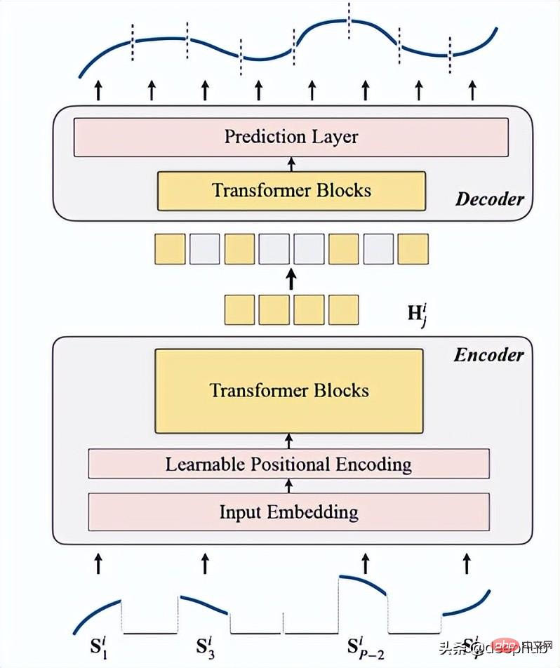
TSFormer is basically similar to the main architecture of MAE, data Passed through an encoder and then through a decoder, the final goal is to reconstruct the missing (artificially masked) data.

We summarize it into the following four points:
1. Masking
is used as the first step before data enters the encoder. The input sequence (Sᶦ) has been distributed into P slices, whose length is L. Therefore, the langth of the sliding window used to predict the next time step is P XL.

The occlusion ratio is 75% (it looks very high, probably because it uses the same parameters as MAE); What we want to complete is a self-supervised task, so the higher the data The fewer encoders the faster the calculation.
The main reason for doing this (masking input sequence segments) is that
- segments (patch) are better than individual points.
- It makes it simple to use downstream models (STGNN takes unit segments as input)
- It can decompose the input size of the encoder.
class Patch(nn.Module):<br>def __init__(self, patch_size, input_channel, output_channel, spectral=True):<br>super().__init__()<br>self.output_channel = output_channel<br>self.P = patch_size<br>self.input_channel = input_channel<br>self.output_channel = output_channel<br>self.spectral = spectral<br>if spectral:<br>self.emb_layer = nn.Linear(int(patch_size/2+1)*2, output_channel)<br>else:<br>self.input_embedding = nn.Conv2d(input_channel, output_channel, kernel_size=(self.P, 1), stride=(self.P, 1))<br>def forward(self, input):<br>B, N, C, L = input.shape<br>if self.spectral:<br>spec_feat_ = torch.fft.rfft(input.unfold(-1, self.P, self.P), dim=-1)<br>real = spec_feat_.real<br>imag = spec_feat_.imag<br>spec_feat = torch.cat([real, imag], dim=-1).squeeze(2)<br>output = self.emb_layer(spec_feat).transpose(-1, -2)<br>else:<br>input = input.unsqueeze(-1) # B, N, C, L, 1<br>input = input.reshape(B*N, C, L, 1) # B*N, C, L, 1<br>output = self.input_embedding(input) # B*N, d, L/P, 1<br>output = output.squeeze(-1).view(B, N, self.output_channel, -1)<br>assert output.shape[-1] == L / self.P<br>return output
The following is the function to generate masking:
class MaskGenerator(nn.Module):<br>def __init__(self, mask_size, mask_ratio, distribution='uniform', lm=-1):<br>super().__init__()<br>self.mask_size = mask_size<br>self.mask_ratio = mask_ratio<br>self.sort = True<br>self.average_patch = lm<br>self.distribution = distribution<br>if self.distribution == "geom":<br>assert lm != -1<br>assert distribution in ['geom', 'uniform']<br>def uniform_rand(self):<br>mask = list(range(int(self.mask_size)))<br>random.shuffle(mask)<br>mask_len = int(self.mask_size * self.mask_ratio)<br>self.masked_tokens = mask[:mask_len]<br>self.unmasked_tokens = mask[mask_len:]<br>if self.sort:<br>self.masked_tokens = sorted(self.masked_tokens)<br>self.unmasked_tokens = sorted(self.unmasked_tokens)<br>return self.unmasked_tokens, self.masked_tokens<br>def geometric_rand(self):<br>mask = geom_noise_mask_single(self.mask_size, lm=self.average_patch, masking_ratio=self.mask_ratio) # 1: masked, 0:unmasked<br>self.masked_tokens = np.where(mask)[0].tolist()<br>self.unmasked_tokens = np.where(~mask)[0].tolist()<br># assert len(self.masked_tokens) > len(self.unmasked_tokens)<br>return self.unmasked_tokens, self.masked_tokens<br>def forward(self):<br>if self.distribution == 'geom':<br>self.unmasked_tokens, self.masked_tokens = self.geometric_rand()<br>elif self.distribution == 'uniform':<br>self.unmasked_tokens, self.masked_tokens = self.uniform_rand()<br>else:<br>raise Exception("ERROR")<br>return self.unmasked_tokens, self.masked_tokens2. Encoding
Includes input embedding, position encoding and Transformer block. The encoder can only be executed on unmasked patches (this is also the MAE method).
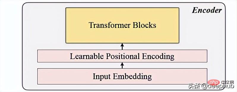
Input embedding
Uses linear projection to obtain the input embedding, which converts the unmasked space into a latent space. Its formula can be seen below:

W and B are the learnable parameters and U is the model input vector in dimension.
Positional encoding
A simple positional encoding layer is used to append new sequence information. Added the word "learnable", which helps show better performance than sine. Hence learnable location embeddings show good results for time series.
class LearnableTemporalPositionalEncoding(nn.Module):<br>def __init__(self, d_model, dropout=0.1, max_len: int = 1000):<br>super().__init__()<br>self.dropout = nn.Dropout(p=dropout)<br>self.pe = nn.Parameter(torch.empty(max_len, d_model), requires_grad=True)<br>nn.init.uniform_(self.pe, -0.02, 0.02)<br><br>def forward(self, X, index):<br>if index is None:<br>pe = self.pe[:X.size(1), :].unsqueeze(0)<br>else:<br>pe = self.pe[index].unsqueeze(0)<br>X = X + pe<br>X = self.dropout(X)<br>return X<br>class PositionalEncoding(nn.Module):<br>def __init__(self, hidden_dim, dropout=0.1):<br>super().__init__()<br>self.tem_pe = LearnableTemporalPositionalEncoding(hidden_dim, dropout)<br>def forward(self, input, index=None, abs_idx=None):<br>B, N, L_P, d = input.shape<br># temporal embedding<br>input = self.tem_pe(input.view(B*N, L_P, d), index=index)<br>input = input.view(B, N, L_P, d)<br># absolute positional embedding<br>return input
Transformer block
The paper uses 4 layers of Transformer, which is a lower number than is common in computer vision and natural language processing tasks. The Transformer used here is the most basic structure mentioned in the original paper, as shown in Figure 4 below:
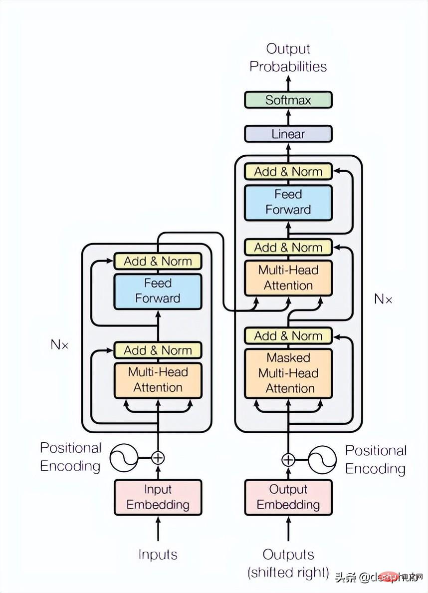
class TransformerLayers(nn.Module):<br>def __init__(self, hidden_dim, nlayers, num_heads=4, dropout=0.1):<br>super().__init__()<br>self.d_model = hidden_dim<br>encoder_layers = TransformerEncoderLayer(hidden_dim, num_heads, hidden_dim*4, dropout)<br>self.transformer_encoder = TransformerEncoder(encoder_layers, nlayers)<br>def forward(self, src):<br>B, N, L, D = src.shape<br>src = src * math.sqrt(self.d_model)<br>src = src.view(B*N, L, D)<br>src = src.transpose(0, 1)<br>output = self.transformer_encoder(src, mask=None)<br>output = output.transpose(0, 1).view(B, N, L, D)<br>return output
3, decoding

The decoder consists of a series of Transformer blocks. It applies to all patches (in contrast, MAE has no position embedding, because its patches already have position information), and the number of layers is only one, and then uses a simple MLP, which makes the output length equal to each patch. length.
4. Reconstruction target

Calculate the masking patch for each data point (i), and select mae (Mean-Absolute-Error) as Loss functions for the main sequence and the reconstructed sequence.
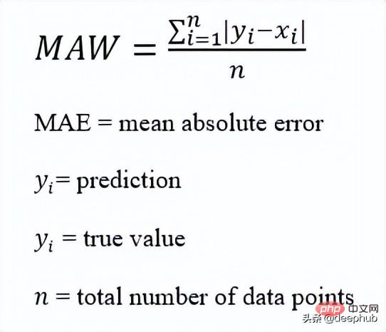
This is the overall architecture
The following is the code implementation:
def trunc_normal_(tensor, mean=0., std=1.):<br>__call_trunc_normal_(tensor, mean=mean, std=std, a=-std, b=std)<br>def unshuffle(shuffled_tokens):<br>dic = {}<br>for k, v, in enumerate(shuffled_tokens):<br>dic[v] = k<br>unshuffle_index = []<br>for i in range(len(shuffled_tokens)):<br>unshuffle_index.append(dic[i])<br>return unshuffle_index<br>class TSFormer(nn.Module):<br>def __init__(self, patch_size, in_channel, out_channel, dropout, mask_size, mask_ratio, L=6, distribution='uniform', lm=-1, selected_feature=0, mode='Pretrain', spectral=True):<br>super().__init__()<br>self.patch_size = patch_size<br>self.seleted_feature = selected_feature<br>self.mode = mode<br>self.spectral = spectral<br>self.patch = Patch(patch_size, in_channel, out_channel, spectral=spectral)<br>self.pe = PositionalEncoding(out_channel, dropout=dropout)<br>self.mask = MaskGenerator(mask_size, mask_ratio, distribution=distribution, lm=lm)<br>self.encoder = TransformerLayers(out_channel, L)<br>self.decoder = TransformerLayers(out_channel, 1)<br>self.encoder_2_decoder = nn.Linear(out_channel, out_channel)<br>self.mask_token = nn.Parameter(torch.zeros(1, 1, 1, out_channel))<br>trunc_normal_(self.mask_token, std=.02)<br>if self.spectral:<br>self.output_layer = nn.Linear(out_channel, int(patch_size/2+1)*2)<br>else:<br>self.output_layer = nn.Linear(out_channel, patch_size)<br>def _forward_pretrain(self, input):<br>B, N, C, L = input.shape<br># get patches and exec input embedding<br>patches = self.patch(input) <br>patches = patches.transpose(-1, -2) <br># positional embedding<br>patches = self.pe(patches)<br><br># mask tokens<br>unmasked_token_index, masked_token_index = self.mask()<br>encoder_input = patches[:, :, unmasked_token_index, :] <br># encoder<br>H = self.encoder(encoder_input) <br># encoder to decoder<br>H = self.encoder_2_decoder(H)<br># decoder<br># H_unmasked = self.pe(H, index=unmasked_token_index)<br>H_unmasked = H<br>H_masked = self.pe(self.mask_token.expand(B, N, len(masked_token_index), H.shape[-1]), index=masked_token_index)<br>H_full = torch.cat([H_unmasked, H_masked], dim=-2) # # B, N, L/P, d<br>H = self.decoder(H_full)<br># output layer<br>if self.spectral:<br># output = H<br>spec_feat_H_ = self.output_layer(H)<br>real = spec_feat_H_[..., :int(self.patch_size/2+1)]<br>imag = spec_feat_H_[..., int(self.patch_size/2+1):]<br>spec_feat_H = torch.complex(real, imag)<br>out_full = torch.fft.irfft(spec_feat_H)<br>else:<br>out_full = self.output_layer(H)<br># prepare loss<br>B, N, _, _ = out_full.shape <br>out_masked_tokens = out_full[:, :, len(unmasked_token_index):, :]<br>out_masked_tokens = out_masked_tokens.view(B, N, -1).transpose(1, 2)<br>label_full = input.permute(0, 3, 1, 2).unfold(1, self.patch_size, self.patch_size)[:, :, :, self.seleted_feature, :].transpose(1, 2) # B, N, L/P, P<br>label_masked_tokens = label_full[:, :, masked_token_index, :].contiguous()<br>label_masked_tokens = label_masked_tokens.view(B, N, -1).transpose(1, 2)<br># prepare plot<br>## note that the output_full and label_full are not aligned. The out_full in shuffled<br>### therefore, unshuffle for plot<br>unshuffled_index = unshuffle(unmasked_token_index + masked_token_index)<br>out_full_unshuffled = out_full[:, :, unshuffled_index, :]<br>plot_args = {}<br>plot_args['out_full_unshuffled'] = out_full_unshuffled<br>plot_args['label_full'] = label_full<br>plot_args['unmasked_token_index'] = unmasked_token_index<br>plot_args['masked_token_index'] = masked_token_index<br>return out_masked_tokens, label_masked_tokens, plot_args<br>def _forward_backend(self, input):<br>B, N, C, L = input.shape<br># get patches and exec input embedding<br>patches = self.patch(input) <br>patches = patches.transpose(-1, -2) <br># positional embedding<br>patches = self.pe(patches)<br>encoder_input = patches # no mask when running the backend.<br># encoder<br>H = self.encoder(encoder_input) <br>return H<br>def forward(self, input_data):<br><br>if self.mode == 'Pretrain':<br>return self._forward_pretrain(input_data)<br>else:<br>return self._forward_backend(input_data)After reading In this paper, I found that it basically replicates MAE, or MAE of time series. The prediction stage is similar to MAE. It uses the output of the encoder as a feature and provides feature data as input for downstream tasks. I am interested. You can read the original paper and look at the code provided in the paper.
The above is the detailed content of Comparison summary of five deep learning models for time series forecasting. For more information, please follow other related articles on the PHP Chinese website!

Hot AI Tools

Undresser.AI Undress
AI-powered app for creating realistic nude photos

AI Clothes Remover
Online AI tool for removing clothes from photos.

Undress AI Tool
Undress images for free

Clothoff.io
AI clothes remover

AI Hentai Generator
Generate AI Hentai for free.

Hot Article

Hot Tools

Notepad++7.3.1
Easy-to-use and free code editor

SublimeText3 Chinese version
Chinese version, very easy to use

Zend Studio 13.0.1
Powerful PHP integrated development environment

Dreamweaver CS6
Visual web development tools

SublimeText3 Mac version
God-level code editing software (SublimeText3)

Hot Topics
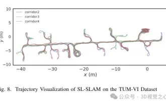 Beyond ORB-SLAM3! SL-SLAM: Low light, severe jitter and weak texture scenes are all handled
May 30, 2024 am 09:35 AM
Written previously, today we discuss how deep learning technology can improve the performance of vision-based SLAM (simultaneous localization and mapping) in complex environments. By combining deep feature extraction and depth matching methods, here we introduce a versatile hybrid visual SLAM system designed to improve adaptation in challenging scenarios such as low-light conditions, dynamic lighting, weakly textured areas, and severe jitter. sex. Our system supports multiple modes, including extended monocular, stereo, monocular-inertial, and stereo-inertial configurations. In addition, it also analyzes how to combine visual SLAM with deep learning methods to inspire other research. Through extensive experiments on public datasets and self-sampled data, we demonstrate the superiority of SL-SLAM in terms of positioning accuracy and tracking robustness.
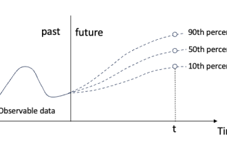 Quantile regression for time series probabilistic forecasting
May 07, 2024 pm 05:04 PM
Do not change the meaning of the original content, fine-tune the content, rewrite the content, and do not continue. "Quantile regression meets this need, providing prediction intervals with quantified chances. It is a statistical technique used to model the relationship between a predictor variable and a response variable, especially when the conditional distribution of the response variable is of interest When. Unlike traditional regression methods, quantile regression focuses on estimating the conditional magnitude of the response variable rather than the conditional mean. "Figure (A): Quantile regression Quantile regression is an estimate. A modeling method for the linear relationship between a set of regressors X and the quantiles of the explained variables Y. The existing regression model is actually a method to study the relationship between the explained variable and the explanatory variable. They focus on the relationship between explanatory variables and explained variables
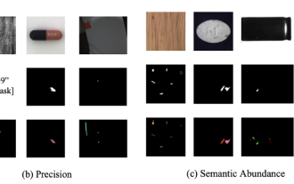 Breaking through the boundaries of traditional defect detection, 'Defect Spectrum' achieves ultra-high-precision and rich semantic industrial defect detection for the first time.
Jul 26, 2024 pm 05:38 PM
In modern manufacturing, accurate defect detection is not only the key to ensuring product quality, but also the core of improving production efficiency. However, existing defect detection datasets often lack the accuracy and semantic richness required for practical applications, resulting in models unable to identify specific defect categories or locations. In order to solve this problem, a top research team composed of Hong Kong University of Science and Technology Guangzhou and Simou Technology innovatively developed the "DefectSpectrum" data set, which provides detailed and semantically rich large-scale annotation of industrial defects. As shown in Table 1, compared with other industrial data sets, the "DefectSpectrum" data set provides the most defect annotations (5438 defect samples) and the most detailed defect classification (125 defect categories
 NVIDIA dialogue model ChatQA has evolved to version 2.0, with the context length mentioned at 128K
Jul 26, 2024 am 08:40 AM
The open LLM community is an era when a hundred flowers bloom and compete. You can see Llama-3-70B-Instruct, QWen2-72B-Instruct, Nemotron-4-340B-Instruct, Mixtral-8x22BInstruct-v0.1 and many other excellent performers. Model. However, compared with proprietary large models represented by GPT-4-Turbo, open models still have significant gaps in many fields. In addition to general models, some open models that specialize in key areas have been developed, such as DeepSeek-Coder-V2 for programming and mathematics, and InternVL for visual-language tasks.
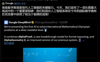 Google AI won the IMO Mathematical Olympiad silver medal, the mathematical reasoning model AlphaProof was launched, and reinforcement learning is so back
Jul 26, 2024 pm 02:40 PM
For AI, Mathematical Olympiad is no longer a problem. On Thursday, Google DeepMind's artificial intelligence completed a feat: using AI to solve the real question of this year's International Mathematical Olympiad IMO, and it was just one step away from winning the gold medal. The IMO competition that just ended last week had six questions involving algebra, combinatorics, geometry and number theory. The hybrid AI system proposed by Google got four questions right and scored 28 points, reaching the silver medal level. Earlier this month, UCLA tenured professor Terence Tao had just promoted the AI Mathematical Olympiad (AIMO Progress Award) with a million-dollar prize. Unexpectedly, the level of AI problem solving had improved to this level before July. Do the questions simultaneously on IMO. The most difficult thing to do correctly is IMO, which has the longest history, the largest scale, and the most negative
 Training with millions of crystal data to solve the crystallographic phase problem, the deep learning method PhAI is published in Science
Aug 08, 2024 pm 09:22 PM
Editor |KX To this day, the structural detail and precision determined by crystallography, from simple metals to large membrane proteins, are unmatched by any other method. However, the biggest challenge, the so-called phase problem, remains retrieving phase information from experimentally determined amplitudes. Researchers at the University of Copenhagen in Denmark have developed a deep learning method called PhAI to solve crystal phase problems. A deep learning neural network trained using millions of artificial crystal structures and their corresponding synthetic diffraction data can generate accurate electron density maps. The study shows that this deep learning-based ab initio structural solution method can solve the phase problem at a resolution of only 2 Angstroms, which is equivalent to only 10% to 20% of the data available at atomic resolution, while traditional ab initio Calculation
 Nature's point of view: The testing of artificial intelligence in medicine is in chaos. What should be done?
Aug 22, 2024 pm 04:37 PM
Editor | ScienceAI Based on limited clinical data, hundreds of medical algorithms have been approved. Scientists are debating who should test the tools and how best to do so. Devin Singh witnessed a pediatric patient in the emergency room suffer cardiac arrest while waiting for treatment for a long time, which prompted him to explore the application of AI to shorten wait times. Using triage data from SickKids emergency rooms, Singh and colleagues built a series of AI models that provide potential diagnoses and recommend tests. One study showed that these models can speed up doctor visits by 22.3%, speeding up the processing of results by nearly 3 hours per patient requiring a medical test. However, the success of artificial intelligence algorithms in research only verifies this
 To provide a new scientific and complex question answering benchmark and evaluation system for large models, UNSW, Argonne, University of Chicago and other institutions jointly launched the SciQAG framework
Jul 25, 2024 am 06:42 AM
Editor |ScienceAI Question Answering (QA) data set plays a vital role in promoting natural language processing (NLP) research. High-quality QA data sets can not only be used to fine-tune models, but also effectively evaluate the capabilities of large language models (LLM), especially the ability to understand and reason about scientific knowledge. Although there are currently many scientific QA data sets covering medicine, chemistry, biology and other fields, these data sets still have some shortcomings. First, the data form is relatively simple, most of which are multiple-choice questions. They are easy to evaluate, but limit the model's answer selection range and cannot fully test the model's ability to answer scientific questions. In contrast, open-ended Q&A


