 Technology peripherals
 AI
AI
 Full code example of deep learning for medical images: Segmenting images from MRI brain scans using Pytorch
Full code example of deep learning for medical images: Segmenting images from MRI brain scans using Pytorch
Image segmentation is one of the most important tasks in medical image analysis, and is often the first and most critical step in many clinical applications. In brain MRI analysis, image segmentation is commonly used to measure and visualize anatomical structures, analyze brain changes, delineate pathological areas, and surgical planning and image-guided interventions. Segmentation is a prerequisite for most morphological analyses.
In this article we will introduce how to use QuickNAT to segment images of the human brain. Use MONAI, PyTorch and common Python libraries for data visualization and calculations such as NumPy, TorchIO and matplotlib.
This article will mainly design the following aspects:
- Setting up the data set and exploring the data
- Processing and preparing the data set for appropriate model training
- Create a training loop
- Evaluate the model and analyze the results
The complete code will be provided at the end of this article.
Set the data directory
The first step to use MONAI is to set the MONAI_DATA_DIRECTORY environment variable to specify the directory. If not specified, a temporary directory will be used.
<code>directory = os.environ.get("MONAI_DATA_DIRECTORY") root_dir = tempfile.mkdtemp() if directory is None else directory print(root_dir)</code>Set up the dataset
One of the main challenges in scaling CNN models to brain segmentation is the limited availability of human-annotated training data. The authors introduce a new training strategy that utilizes large datasets without manual labels and small datasets with manual labels.
First, use existing software tools (such as FreeSurfer) to obtain automatically generated segmentations from large unlabeled datasets, and then use these tools to pre-train the network. In the second step, the network is fine-tuned using smaller manually annotated data [2].
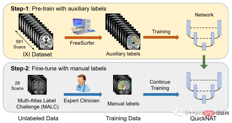
The IXI dataset consists of 581 unlabeled MRI T1 scans of healthy subjects. The data was collected from 3 different hospitals in London. The main disadvantage of using this dataset is that the labels are not publicly available, so in order to follow the same approach as in the research paper, this article will use FreeSurfer to generate segmentations for these MRI T1 scans.
FreeSurfer is a software package for analyzing and visualizing structures. Download and installation instructions can be found here. All cortical reconstruction processes can be performed directly using the "recon-all" command.
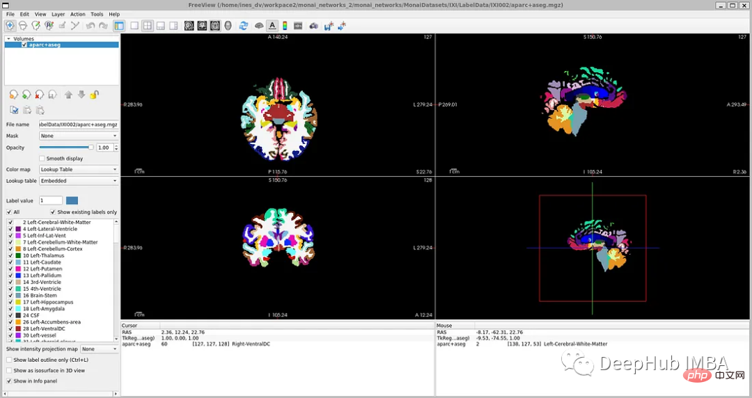
Although FreeSurfer is a very useful tool for leveraging large amounts of unlabeled data and training networks in a supervised manner, scanning to generate these labels requires up to 5 hours, so here we train the model directly using the OASIS dataset, which is a smaller dataset with publicly available manual annotations.
OASIS is a project to make brain neuroimaging datasets freely available to the scientific community. OASIS-1 is a dataset consisting of cross-sections of 39 subjects, obtained as follows:
<code>resource = "https://download.nrg.wustl.edu/data/oasis_cross-sectional_disc1.tar.gz" md5 = "c83e216ef8654a7cc9e2a30a4cdbe0cc" compressed_file = os.path.join(root_dir, "oasis_cross-sectional_disc1.tar.gz") data_dir = os.path.join(root_dir, "Oasis_Data") if not os.path.exists(data_dir): download_and_extract(resource, compressed_file, data_dir, md5)</code>
Data Exploration
If you open 'oasis_crosssectional_disc1.tar.gz', you will Found that each theme has different folders. For example, for the topic OAS1_0001_MR1, it is like this:
Mirror data file path: disc1\OAS1_0001_MR1\PROCESSED\MPRAGE\T88_111\ oas1_0001_mr1_mpr_n4_anon_111_t88_masked_ggc .img
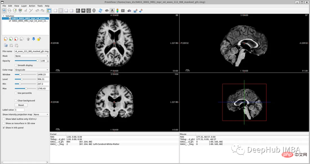
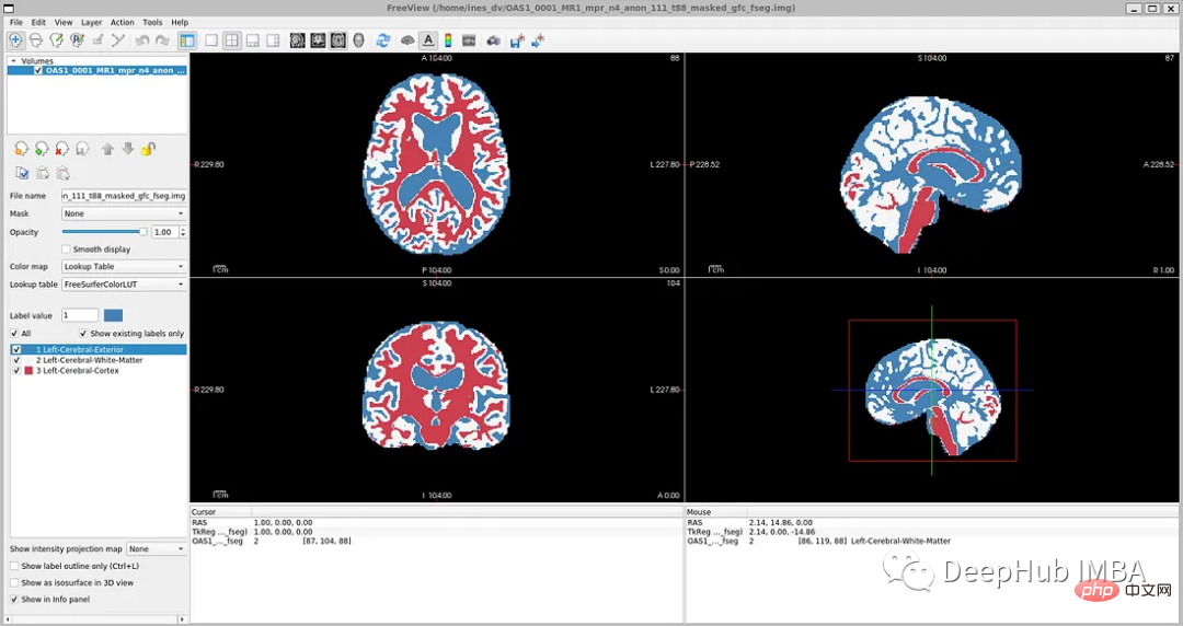
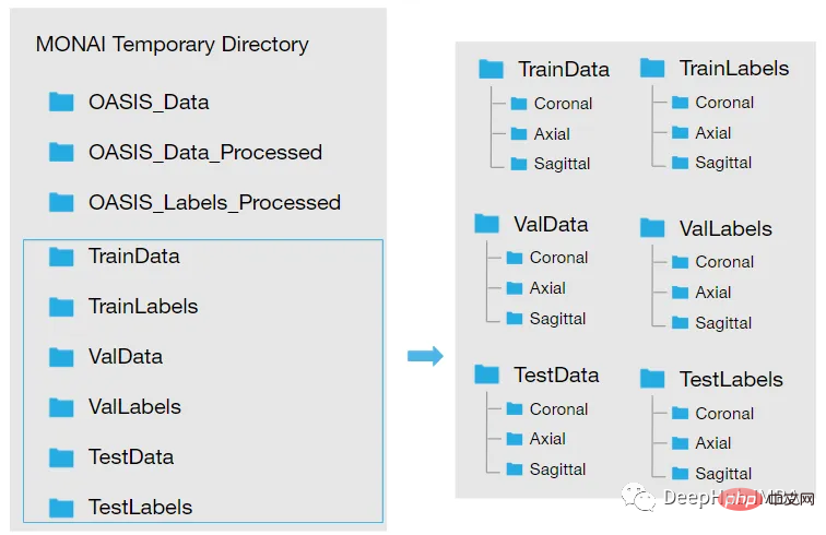
<code>new_path_data= root_dir + '/Oasis_Data_Processed/' if not os.path.exists(new_path_data): os.makedirs(new_path_data) new_path_labels= root_dir + '/Oasis_Labels_Processed/' if not os.path.exists(new_path_labels): os.makedirs(new_path_labels)</code>
<code>for i in [x for x in range(1, 43) if x != 8 and x != 24 and x != 36]: if i </code>
<code>image_files = sorted(glob(os.path.join(root_dir + '/Oasis_Data_Processed', '*.nii'))) label_files = sorted(glob(os.path.join(root_dir + '/Oasis_Labels_Processed', '*.nii'))) files = [{'image': image_name, 'label': label_name} for image_name, label_name in zip(image_files, label_files)]</code><code>image_filename = root_dir + '/Oasis_Data_Processed/OAS1_0001_MR1_mpr_n4_anon_111_t88_masked_gfc.nii' label_filename = root_dir + '/Oasis_Labels_Processed/OAS1_0001_MR1_mpr_n4_anon_111_t88_masked_gfc_fseg.nii' subject = torchio.Subject(image=torchio.ScalarImage(image_filename), label=torchio.LabelMap(label_filename)) subject.plot()</code>
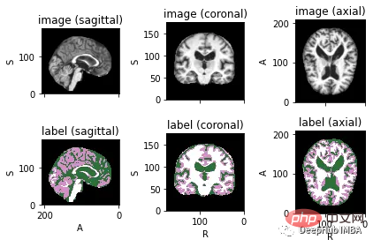
下面就是将数据分成3部分——训练、验证和测试。将数据分成三个不同的类别的目的是建立一个可靠的机器学习模型,避免过拟合。
我们将整个数据集分成三个部分:
Train: 80%,Validation: 10%,Test: 10%
<code>train_inds, val_inds, test_inds = partition_dataset(data = np.arange(len(files)), ratios = [8, 1, 1], shuffle = True) train = [files[i] for i in sorted(train_inds)] val = [files[i] for i in sorted(val_inds)] test = [files[i] for i in sorted(test_inds)] print(f"Training count: {len(train)}, Validation count: {len(val)}, Test count: {len(test)}")</code>因为模型需要的是二维切片,所以将每个切片保存在不同的文件夹中,如下图所示。这两个代码单元将训练集的每个MRI体积的切片保存为“.png”格式。
<code>Save coronal slices for training images dir = root_dir + '/TrainData' os.makedirs(os.path.join(dir, "Coronal")) path = root_dir + '/TrainData/Coronal/' for file in sorted(glob(os.path.join(root_dir + '/TrainData', '*.nii'))): image=torchio.ScalarImage(file) data = image.data filename = os.path.basename(file) filename = os.path.splitext(filename) for i in range(0, 208): slice = data[0, :, i] array = slice.numpy() data_dir = root_dir + '/TrainData/Coronal/' + filename[0] + '_slice' + str(i) + '.png' plt.imsave(fname = data_dir, arr = array, format = 'png', cmap = plt.cm.gray)</code>
同理,下面是保存标签:
<code>dir = root_dir + '/TrainLabels' os.makedirs(os.path.join(dir, "Coronal")) path = root_dir + '/TrainLabels/Coronal/' for file in sorted(glob(os.path.join(root_dir + '/TrainLabels', '*.nii'))): label = torchio.LabelMap(file) data = label.data filename = os.path.basename(file) filename = os.path.splitext(filename) for i in range(0, 208): slice = data[0, :, i] array = slice.numpy() data_dir = root_dir + '/TrainLabels/Coronal/' + filename[0] + '_slice' + str(i) + '.png' plt.imsave(fname = data_dir, arr = array, format = 'png')</code>
为训练和验证定义图像的变换处理
在本例中,我们将使用Dictionary Transforms,其中数据是Python字典。
<code>train_images_coronal = [] for file in sorted(glob(os.path.join(root_dir + '/TrainData/Coronal', '*.png'))): train_images_coronal.append(file) train_images_coronal = natsort.natsorted(train_images_coronal) train_labels_coronal = [] for file in sorted(glob(os.path.join(root_dir + '/TrainLabels/Coronal', '*.png'))): train_labels_coronal.append(file) train_labels_coronal= natsort.natsorted(train_labels_coronal) val_images_coronal = [] for file in sorted(glob(os.path.join(root_dir + '/ValData/Coronal', '*.png'))): val_images_coronal.append(file) val_images_coronal = natsort.natsorted(val_images_coronal) val_labels_coronal = [] for file in sorted(glob(os.path.join(root_dir + '/ValLabels/Coronal', '*.png'))): val_labels_coronal.append(file) val_labels_coronal = natsort.natsorted(val_labels_coronal) train_files_coronal = [{'image': image_name, 'label': label_name} for image_name, label_name in zip(train_images_coronal, train_labels_coronal)] val_files_coronal = [{'image': image_name, 'label': label_name} for image_name, label_name in zip(val_images_coronal, val_labels_coronal)]</code>现在我们将应用以下变换:
LoadImaged:加载图像数据和元数据。我们使用' PILReader '来加载图像和标签文件。ensure_channel_first设置为True,将图像数组形状转换为通道优先。
Rotate90d:我们将图像和标签旋转90度,因为当我们下载它们时,它们方向是不正确的。
ToTensord:将输入的图像和标签转换为张量。
NormalizeIntensityd:对输入进行规范化。
<code>train_transforms = Compose([ LoadImaged(keys = ['image', 'label'], reader=PILReader(converter=lambda image: image.convert("L")), ensure_channel_first = True), Rotate90d(keys = ['image', 'label'], k = 2), ToTensord(keys = ['image', 'label']), NormalizeIntensityd(keys = ['image'])]) val_transforms = Compose([ LoadImaged(keys = ['image', 'label'], reader=PILReader(converter=lambda image: image.convert("L")), ensure_channel_first = True), Rotate90d(keys = ['image', 'label'], k = 2), ToTensord(keys = ['image', 'label']), NormalizeIntensityd(keys = ['image'])])</code>MaskColorMap将我们定义了一个新的转换,将相应的像素值以一种格式映射为多个标签。这种转换在语义分割中是必不可少的,因为我们必须为每个可能的类别提供二元特征。One-Hot Encoding将对应于原始类别的每个样本的特征赋值为1。
因为OASIS-1数据集只有3个大脑结构标签,对于更详细的分割,理想的情况是像他们在研究论文中那样对28个皮质结构进行注释。在OASIS-1下载说明中,可以找到使用FreeSurfer获得的更多大脑结构的标签。
所以本文将分割更多的神经解剖结构。我们要将模型的参数num_classes修改为相应的标签数量,以便模型的输出是具有N个通道的特征映射,等于num_classes。
为了简化本教程,我们将使用以下标签,比OASIS-1但是要比FreeSurfer的少:
- Label 0: Background
- Label 1: LeftCerebralExterior
- Label 2: LeftWhiteMatter
- Label 3: LeftCerebralCortex
所以MaskColorMap的代码如下:
<code>class MaskColorMap(Enum):Background = (30)LeftCerebralExterior = (91)LeftWhiteMatter = (137)LeftCerebralCortex = (215)</code>
数据集和数据加载
数据集和数据加载器从存储中提取数据,并将其分批发送给训练循环。这里我们使用monai.data.Dataset加载之前定义的训练和验证字典,并对输入数据应用相应的转换。dataloader用于将数据集加载到内存中。我们将为训练和验证以及每个视图定义一个数据集和数据加载器。
为了方便演示,我们使用通过使用torch.utils.data.Subset,在指定的索引处创建一个子集,只是用部分数据训练加快演示速度。
<code>train_dataset_coronal = Dataset(data=train_files_coronal, transform = train_transforms) train_loader_coronal = DataLoader(train_dataset_coronal, batch_size = 1, shuffle = True) val_dataset_coronal = Dataset(data = val_files_coronal, transform = val_transforms) val_loader_coronal = DataLoader(val_dataset_coronal, batch_size = 1, shuffle = False) # We will use a subset of the dataset subset_train = list(range(90, len(train_dataset_coronal), 120)) train_dataset_coronal_subset = torch.utils.data.Subset(train_dataset_coronal, subset_train) train_loader_coronal_subset = DataLoader(train_dataset_coronal_subset, batch_size = 1, shuffle = True) subset_val = list(range(90, len(val_dataset_coronal), 50)) val_dataset_coronal_subset = torch.utils.data.Subset(val_dataset_coronal, subset_val) val_loader_coronal_subset = DataLoader(val_dataset_coronal_subset, batch_size = 1, shuffle = False)</code>
定义模型
给定一组MRI脑扫描I = {I1,…In}及其对应的分割S = {S1,…Sn},我们想要学习一个函数fseg: I -> S。我们将这个函数表示为F-CNN模型,称为QuickNAT:
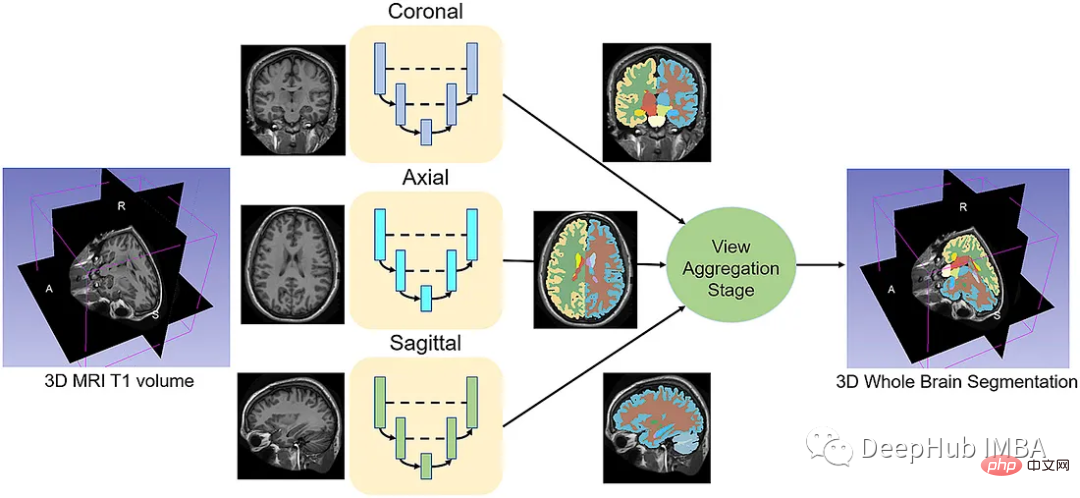
QuickNAT由三个二维f - cnn组成,分别在coronal, axial, sagittal视图上操作,然后通过聚合步骤推断最终的分割结果,该分割结果由三个网络的概率图组合而成。每个F-CNN都有一个编码器/解码器架构,其中有4个编码器和4个解码器,并由瓶颈层分隔。最后一层是带有softmax的分类器块。该架构还包括每个编码器/解码器块内的残差链接。
<code>class QuickNat(nn.Module): """A PyTorch implementation of QuickNAT """ def __init__(self, params): """:param params: {'num_channels':1,'num_filters':64,'kernel_h':5,'kernel_w':5,'stride_conv':1,'pool':2,'stride_pool':2,'num_classes':28'se_block': False,'drop_out':0.2}""" super(QuickNat, self).__init__() # from monai.networks.blocks import squeeze_and_excitation as se # self.cSE = ChannelSELayer(num_channels, reduction_ratio) # self.encode1 = sm.EncoderBlock(params, se_block_type=se.SELayer.CSSE) # params["num_channels"] = params["num_filters"] # self.encode2 = sm.EncoderBlock(params, se_block_type=se.SELayer.CSSE) # self.encode3 = sm.EncoderBlock(params, se_block_type=se.SELayer.CSSE) # self.encode4 = sm.EncoderBlock(params, se_block_type=se.SELayer.CSSE) # self.bottleneck = sm.DenseBlock(params, se_block_type=se.SELayer.CSSE) # params["num_channels"] = params["num_filters"] * 2 # self.decode1 = sm.DecoderBlock(params, se_block_type=se.SELayer.CSSE) # self.decode2 = sm.DecoderBlock(params, se_block_type=se.SELayer.CSSE) # self.decode3 = sm.DecoderBlock(params, se_block_type=se.SELayer.CSSE) # self.decode4 = sm.DecoderBlock(params, se_block_type=se.SELayer.CSSE) # self.encode1 = EncoderBlock(params, se_block_type=se.ChannelSELayer) self.encode1 = EncoderBlock(params, se_block_type=se.SELayer.CSSE) params["num_channels"] = params["num_filters"] self.encode2 = EncoderBlock(params, se_block_type=se.SELayer.CSSE) self.encode3 = EncoderBlock(params, se_block_type=se.SELayer.CSSE) self.encode4 = EncoderBlock(params, se_block_type=se.SELayer.CSSE) self.bottleneck = DenseBlock(params, se_block_type=se.SELayer.CSSE) params["num_channels"] = params["num_filters"] * 2 self.decode1 = DecoderBlock(params, se_block_type=se.SELayer.CSSE) self.decode2 = DecoderBlock(params, se_block_type=se.SELayer.CSSE) self.decode3 = DecoderBlock(params, se_block_type=se.SELayer.CSSE) self.decode4 = DecoderBlock(params, se_block_type=se.SELayer.CSSE) params["num_channels"] = params["num_filters"] self.classifier = ClassifierBlock(params) def forward(self, input): """:param input: X:return: probabiliy map """ e1, out1, ind1 = self.encode1.forward(input) e2, out2, ind2 = self.encode2.forward(e1) e3, out3, ind3 = self.encode3.forward(e2) e4, out4, ind4 = self.encode4.forward(e3) bn = self.bottleneck.forward(e4) d4 = self.decode4.forward(bn, out4, ind4) d3 = self.decode1.forward(d4, out3, ind3) d2 = self.decode2.forward(d3, out2, ind2) d1 = self.decode3.forward(d2, out1, ind1) prob = self.classifier.forward(d1) return prob def enable_test_dropout(self): """Enables test time drop out for uncertainity:return:""" attr_dict = self.__dict__["_modules"] for i in range(1, 5): encode_block, decode_block = ( attr_dict["encode" + str(i)], attr_dict["decode" + str(i)],) encode_block.drop_out = encode_block.drop_out.apply(nn.Module.train) decode_block.drop_out = decode_block.drop_out.apply(nn.Module.train) @property def is_cuda(self): """Check if model parameters are allocated on the GPU.""" return next(self.parameters()).is_cuda def save(self, path): """Save model with its parameters to the given path. Conventionally thepath should end with '*.model'. Inputs:- path: path string""" print("Saving model... %s" % path) torch.save(self.state_dict(), path) def predict(self, X, device=0, enable_dropout=False): """Predicts the output after the model is trained.Inputs:- X: Volume to be predicted""" self.eval() print("tensor size before transformation", X.shape) if type(X) is np.ndarray: # X = torch.tensor(X, requires_grad=False).type(torch.FloatTensor) X = ( torch.tensor(X, requires_grad=False).type(torch.FloatTensor).cuda(device, non_blocking=True)) elif type(X) is torch.Tensor and not X.is_cuda: X = X.type(torch.FloatTensor).cuda(device, non_blocking=True) print("tensor size ", X.shape) if enable_dropout: self.enable_test_dropout() with torch.no_grad(): out = self.forward(X) max_val, idx = torch.max(out, 1) idx = idx.data.cpu().numpy() prediction = np.squeeze(idx) print("prediction shape", prediction.shape) del X, out, idx, max_val return prediction</code>损失函数
神经网络的训练需要一个损失函数来计算模型误差。训练的目标是最小化预测输出和目标输出之间的损失。我们的模型使用Dice Loss 和Weighted Logistic Loss的联合损失函数进行优化,其中权重补偿数据中的高类不平衡,并鼓励正确分割解剖边界。

优化器
优化算法允许我们继续更新模型的参数并最小化损失函数的值,我们设置了以下的超参数:
学习率:初始设置为0.1,10次后降低1阶。这可以通过学习率调度器来实现。
权重衰减:0.0001。
批量大小:1。
动量:设置为0.95的高值,以补偿由于小批量大小而产生的噪声梯度。
训练网络
现在可以训练模型了。对于QuickNAT需要在3个(coronal, axial, sagittal)2d切片上训练3个模型。然后再聚合步骤中组合三个模型的概率生成最终结果,但是本文中只演示在coronal视图的2D切片上训练一个F-CNN模型,因为其他两个与之类似。
<code>num_epochs = 20 start_epoch = 1 val_interval = 1 train_loss_epoch_values = [] val_loss_epoch_values = [] best_ds_mean = -1 best_ds_mean_epoch = -1 ds_mean_train_values = [] ds_mean_val_values = [] # ds_LCE_values = [] # ds_LWM_values = [] # ds_LCC_values = [] print("START TRAINING. : model name = ", "quicknat") for epoch in range(start_epoch, num_epochs): print("==== Epoch ["+ str(epoch) + " / "+ str(num_epochs)+ "] DONE ====") checkpoint_name = CHECKPOINT_DIR + "/checkpoint_epoch_" + str(epoch) + "." + CHECKPOINT_EXTENSION print(checkpoint_name) state = { "epoch": epoch, "arch": "quicknat", "state_dict": model_coronal.state_dict(), "optimizer": optimizer.state_dict(), "scheduler": scheduler.state_dict(),} save_checkpoint(state = state, filename = checkpoint_name) print("\n==== Epoch [ %d / %d ] START ====" % (epoch, num_epochs)) steps_per_epoch = len(train_dataset_coronal_subset) / train_loader_coronal_subset.batch_size model_coronal.train() train_loss_epoch = 0 val_loss_epoch = 0 step = 0 predictions_train = [] labels_train = [] predictions_val = [] labels_val = [] for i_batch, sample_batched in enumerate(train_loader_coronal_subset): inputs = sample_batched['image'].type(torch.FloatTensor) labels = sample_batched['label'].type(torch.LongTensor) # print(f"Train Input Shape: {inputs.shape}") labels = labels.squeeze(1) _img_channels, _img_height, _img_width = labels.shape encoded_label= np.zeros((_img_height, _img_width, 1)).astype(int) for j, cls in enumerate(MaskColorMap): encoded_label[np.all(labels == cls.value, axis = 0)] = j labels = encoded_label labels = torch.from_numpy(labels) labels = torch.permute(labels, (2, 1, 0)) # print(f"Train Label Shape: {labels.shape}") # plt.title("Train Label") # plt.imshow(labels[0, :, :]) # plt.show() optimizer.zero_grad() outputs = model_coronal(inputs) loss = loss_function(outputs, labels) loss.backward() optimizer.step() scheduler.step() with torch.no_grad(): _, batch_output = torch.max(outputs, dim = 1) # print(f"Train Prediction Shape: {batch_output.shape}") # plt.title("Train Prediction") # plt.imshow(batch_output[0, :, :]) # plt.show() predictions_train.append(batch_output.cpu()) labels_train.append(labels.cpu()) train_loss_epoch += loss.item() print(f"{step}/{len(train_dataset_coronal_subset) // train_loader_coronal_subset.batch_size}, Training_loss: {loss.item():.4f}") step += 1 predictions_train_arr, labels_train_arr = torch.cat(predictions_train), torch.cat(labels_train) # print(predictions_train_arr.shape) dice_metric(predictions_train_arr, labels_train_arr) ds_mean_train = dice_metric.aggregate().item() ds_mean_train_values.append(ds_mean_train) dice_metric.reset() train_loss_epoch /= step train_loss_epoch_values.append(train_loss_epoch) print(f"Epoch {epoch + 1} Train Average Loss: {train_loss_epoch:.4f}") if (epoch + 1) % val_interval == 0: model_coronal.eval() step = 0 with torch.no_grad(): for i_batch, sample_batched in enumerate(val_loader_coronal_subset): inputs = sample_batched['image'].type(torch.FloatTensor) labels = sample_batched['label'].type(torch.LongTensor) # print(f"Val Input Shape: {inputs.shape}") labels = labels.squeeze(1) integer_encoded_labels = [] _img_channels, _img_height, _img_width = labels.shape encoded_label= np.zeros((_img_height, _img_width, 1)).astype(int) for j, cls in enumerate(MaskColorMap): encoded_label[np.all(labels == cls.value, axis = 0)] = j labels = encoded_label labels = torch.from_numpy(labels) labels = torch.permute(labels, (2, 1, 0)) # print(f"Val Label Shape: {labels.shape}") # plt.title("Val Label") # plt.imshow(labels[0, :, :]) # plt.show() val_outputs = model_coronal(inputs) val_loss = loss_function(val_outputs, labels) predicted = torch.argmax(val_outputs, dim = 1) # print(f"Val Prediction Shape: {predicted.shape}") # plt.title("Val Prediction") # plt.imshow(predicted[0, :, :]) # plt.show() predictions_val.append(predicted) labels_val.append(labels) val_loss_epoch += val_loss.item() print(f"{step}/{len(val_dataset_coronal_subset) // val_loader_coronal_subset.batch_size}, Validation_loss: {val_loss.item():.4f}") step += 1 predictions_val_arr, labels_val_arr = torch.cat(predictions_val), torch.cat(labels_val) dice_metric(predictions_val_arr, labels_val_arr) # dice_metric_batch(predictions_val_arr, labels_val_arr) ds_mean_val = dice_metric.aggregate().item() ds_mean_val_values.append(ds_mean_val) # ds_mean_val_batch = dice_metric_batch.aggregate() # ds_LCE = ds_mean_val_batch[0].item() # ds_LCE_values.append(ds_LCE) # ds_LWM = ds_mean_val_batch[1].item() # ds_LWM_values.append(ds_LWM) # ds_LCC = ds_mean_val_batch[2].item() # ds_LCC_values.append(ds_LCC) dice_metric.reset() # dice_metric_batch.reset() if ds_mean_val > best_ds_mean: best_ds_mean = ds_mean_val best_ds_mean_epoch = epoch + 1 torch.save(model_coronal.state_dict(), os.path.join(BESTMODEL_DIR, "best_metric_model_coronal.pth")) print("Saved new best metric model coronal") print( f"Current Epoch: {epoch + 1} Current Mean Dice score is: {ds_mean_val:.4f}" f"\nBest Mean Dice score: {best_ds_mean:.4f} " # f"\nMean Dice score Left Cerebral Exterior: {ds_LCE:.4f} Mean Dice score Left White Matter: {ds_LWM:.4f} Mean Dice score Left Cerebral Cortex: {ds_LCC:.4f} " f"at Epoch: {best_ds_mean_epoch}") val_loss_epoch /= step val_loss_epoch_values.append(val_loss_epoch) print(f"Epoch {epoch + 1} Average Validation Loss: {val_loss_epoch:.4f}") print("FINISH.")</code>代码也是传统的Pytorch的训练步骤,就不详细解释了
绘制损失和精度曲线
训练曲线表示模型的学习情况,验证曲线表示模型泛化到未见实例的情况。我们使用matplotlib来绘制图形。还可以使用TensorBoard,它使理解和调试深度学习程序变得更容易,并且是实时的。
<code>epoch = range(1, num_epochs + 1) # Plot Loss Curves plt.figure(figsize=(18, 6)) plt.subplot(1, 3, 1) plt.plot(epoch, train_loss_epoch_values, label='Training Loss') plt.plot(epoch, val_loss_epoch_values, label='Validation Loss') plt.title('Training and Validation Loss') plt.xlabel('Epoch') plt.legend() plt.figure() plt.show() # Plot Train Dice Coefficient Curve plt.figure(figsize=(18, 6)) plt.subplot(1, 3, 2) x = [(i + 1) for i in range(len(ds_mean_train_values))] plt.plot(x, ds_mean_train_values, 'blue', label = 'Train Mean Dice Score') plt.title("Training Mean Dice Coefficient") plt.xlabel('Epoch') plt.ylabel('Mean Dice Score') plt.show() # Plot Validation Dice Coefficient Curve plt.figure(figsize=(18, 6)) plt.subplot(1, 3, 3) x = [(i + 1) for i in range(len(ds_mean_val_values))] plt.plot(x, ds_mean_val_values, 'orange', label = 'Validation Mean Dice Score') plt.title("Validation Mean Dice Coefficient") plt.xlabel('Epoch') plt.ylabel('Mean Dice Score') plt.show()</code>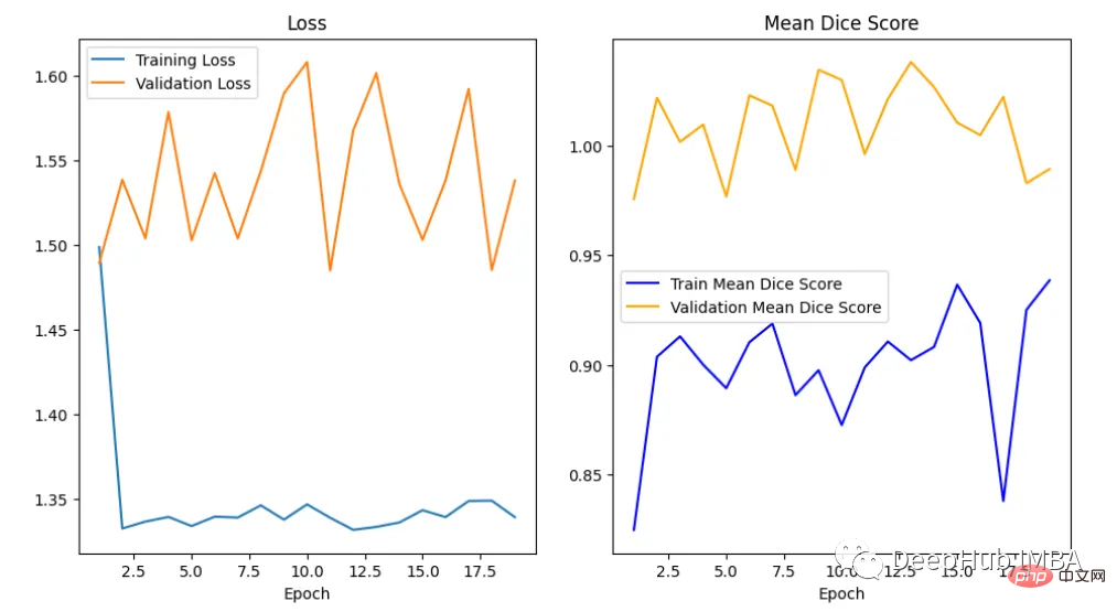
在曲线中,我们可以看到模型是过拟合的,因为验证损失上升而训练损失下降。这是深度学习算法中一个常见的陷阱,其中模型最终会记住训练数据,而无法对未见过的数据进行泛化。
避免过度拟合的技巧:
- 用更多的数据进行训练:更大的数据集可以减少过拟合。
- 数据增强:如果我们不能收集更多的数据,我们可以应用数据增强来人为地增加数据集的大小。
- 添加正则化:正则化是一种限制我们的网络学习过于复杂的模型的技术,因此可能会过度拟合。
评估网络
我们如何度量模型的性能?一个成功的预测是一个最大限度地扩大预测和真实之间的重叠。
这一目标的两个相关但不同的指标是Dice和Intersection / Union (IoU)系数,后者也被称为Jaccard系数。两个指标都在0(无重叠)和1(完全重叠)之间。

这两种指标都可以用于类似的情况,但是区别在于Dice Score倾向于平均表现,而IoU则帮助你理解最坏情况下的表现。

我们可以逐个类地检查度量标准,或者取所有类的平均值。这里将使用monai.metrics.DiceMetric来计算分数。一个更通用的方法是使用torchmetrics,但是因为这里使用了monai框架,所以就直接使用它内置的函数了。
我们可以看到Dice得分曲线的行为相当不寻常。主要是因为验证平均Dice得分高于1,这是不可能的,因为这个度量是在0和1之间。我们无法确定这种行为的主要原因,但我们建议在多类问题中为每个类单独提供度量计算,并始终提供可视化示例以进行可视化评估。
结果分析
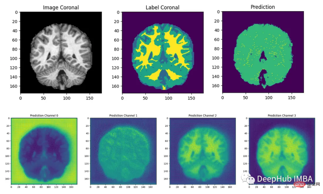
最后我们要看看模型是如何推广到未知数据的这个模型预测的几乎所有东西都是左脑白质,一些像素是左脑皮层。尽管它的预测似乎是正确的,但仍有很大的改进空间,因为我们的模型太小了,可以选择更深的模型获得更好的效果。
总结
在本文中,我们介绍了如何训练QuickNAT来完成具有挑战性的大脑分割任务。我们尽可能遵循作者在他们的研究论文中解释的学习策略,这是本教程为了方便演示只在最简单的步骤上进行了演示,文本的完整代码:
https://github.com/inesdv26/Brain-Segmentation
The above is the detailed content of Full code example of deep learning for medical images: Segmenting images from MRI brain scans using Pytorch. For more information, please follow other related articles on the PHP Chinese website!

Hot AI Tools

Undresser.AI Undress
AI-powered app for creating realistic nude photos

AI Clothes Remover
Online AI tool for removing clothes from photos.

Undress AI Tool
Undress images for free

Clothoff.io
AI clothes remover

AI Hentai Generator
Generate AI Hentai for free.

Hot Article

Hot Tools

Notepad++7.3.1
Easy-to-use and free code editor

SublimeText3 Chinese version
Chinese version, very easy to use

Zend Studio 13.0.1
Powerful PHP integrated development environment

Dreamweaver CS6
Visual web development tools

SublimeText3 Mac version
God-level code editing software (SublimeText3)

Hot Topics
 Methods and steps for using BERT for sentiment analysis in Python
Jan 22, 2024 pm 04:24 PM
BERT is a pre-trained deep learning language model proposed by Google in 2018. The full name is BidirectionalEncoderRepresentationsfromTransformers, which is based on the Transformer architecture and has the characteristics of bidirectional encoding. Compared with traditional one-way coding models, BERT can consider contextual information at the same time when processing text, so it performs well in natural language processing tasks. Its bidirectionality enables BERT to better understand the semantic relationships in sentences, thereby improving the expressive ability of the model. Through pre-training and fine-tuning methods, BERT can be used for various natural language processing tasks, such as sentiment analysis, naming
 Analysis of commonly used AI activation functions: deep learning practice of Sigmoid, Tanh, ReLU and Softmax
Dec 28, 2023 pm 11:35 PM
Activation functions play a crucial role in deep learning. They can introduce nonlinear characteristics into neural networks, allowing the network to better learn and simulate complex input-output relationships. The correct selection and use of activation functions has an important impact on the performance and training results of neural networks. This article will introduce four commonly used activation functions: Sigmoid, Tanh, ReLU and Softmax, starting from the introduction, usage scenarios, advantages, disadvantages and optimization solutions. Dimensions are discussed to provide you with a comprehensive understanding of activation functions. 1. Sigmoid function Introduction to SIgmoid function formula: The Sigmoid function is a commonly used nonlinear function that can map any real number to between 0 and 1. It is usually used to unify the
 Introduction to five sampling methods in natural language generation tasks and Pytorch code implementation
Feb 20, 2024 am 08:50 AM
In natural language generation tasks, sampling method is a technique to obtain text output from a generative model. This article will discuss 5 common methods and implement them using PyTorch. 1. GreedyDecoding In greedy decoding, the generative model predicts the words of the output sequence based on the input sequence time step by time. At each time step, the model calculates the conditional probability distribution of each word, and then selects the word with the highest conditional probability as the output of the current time step. This word becomes the input to the next time step, and the generation process continues until some termination condition is met, such as a sequence of a specified length or a special end marker. The characteristic of GreedyDecoding is that each time the current conditional probability is the best
 Beyond ORB-SLAM3! SL-SLAM: Low light, severe jitter and weak texture scenes are all handled
May 30, 2024 am 09:35 AM
Written previously, today we discuss how deep learning technology can improve the performance of vision-based SLAM (simultaneous localization and mapping) in complex environments. By combining deep feature extraction and depth matching methods, here we introduce a versatile hybrid visual SLAM system designed to improve adaptation in challenging scenarios such as low-light conditions, dynamic lighting, weakly textured areas, and severe jitter. sex. Our system supports multiple modes, including extended monocular, stereo, monocular-inertial, and stereo-inertial configurations. In addition, it also analyzes how to combine visual SLAM with deep learning methods to inspire other research. Through extensive experiments on public datasets and self-sampled data, we demonstrate the superiority of SL-SLAM in terms of positioning accuracy and tracking robustness.
 The perfect combination of PyCharm and PyTorch: detailed installation and configuration steps
Feb 21, 2024 pm 12:00 PM
PyCharm is a powerful integrated development environment (IDE), and PyTorch is a popular open source framework in the field of deep learning. In the field of machine learning and deep learning, using PyCharm and PyTorch for development can greatly improve development efficiency and code quality. This article will introduce in detail how to install and configure PyTorch in PyCharm, and attach specific code examples to help readers better utilize the powerful functions of these two. Step 1: Install PyCharm and Python
 Latent space embedding: explanation and demonstration
Jan 22, 2024 pm 05:30 PM
Latent Space Embedding (LatentSpaceEmbedding) is the process of mapping high-dimensional data to low-dimensional space. In the field of machine learning and deep learning, latent space embedding is usually a neural network model that maps high-dimensional input data into a set of low-dimensional vector representations. This set of vectors is often called "latent vectors" or "latent encodings". The purpose of latent space embedding is to capture important features in the data and represent them into a more concise and understandable form. Through latent space embedding, we can perform operations such as visualizing, classifying, and clustering data in low-dimensional space to better understand and utilize the data. Latent space embedding has wide applications in many fields, such as image generation, feature extraction, dimensionality reduction, etc. Latent space embedding is the main
 Implementing noise removal diffusion model using PyTorch
Jan 14, 2024 pm 10:33 PM
Before we understand the working principle of the Denoising Diffusion Probabilistic Model (DDPM) in detail, let us first understand some of the development of generative artificial intelligence, which is also one of the basic research of DDPM. VAEVAE uses an encoder, a probabilistic latent space, and a decoder. During training, the encoder predicts the mean and variance of each image and samples these values from a Gaussian distribution. The result of the sampling is passed to the decoder, which converts the input image into a form similar to the output image. KL divergence is used to calculate the loss. A significant advantage of VAE is its ability to generate diverse images. In the sampling stage, one can directly sample from the Gaussian distribution and generate new images through the decoder. GAN has made great progress in variational autoencoders (VAEs) in just one year.
 Tutorial on installing PyCharm with PyTorch
Feb 24, 2024 am 10:09 AM
As a powerful deep learning framework, PyTorch is widely used in various machine learning projects. As a powerful Python integrated development environment, PyCharm can also provide good support when implementing deep learning tasks. This article will introduce in detail how to install PyTorch in PyCharm and provide specific code examples to help readers quickly get started using PyTorch for deep learning tasks. Step 1: Install PyCharm First, we need to make sure we have


