Integrated multi-graph neural network

1. GNN from a unified perspective
1. Existing GNN propagation paradigm
How does GNN propagate in the airspace? As shown in the figure below, take node A as an example:
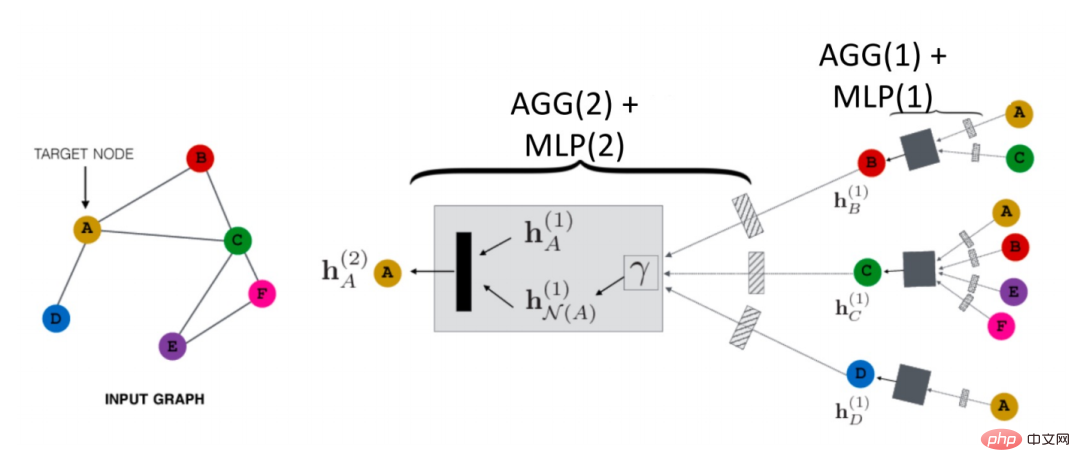
##First it will identify its neighbors The information of node N (A) is aggregated into a hN(A)(1 ), and then combine it with A to represent the upper layer h# #N(A)(1) is combined, and then through a transformation function (i.e. Trans(·) in the formula), the next level representation of A is obtained hN(A)(2). This is the most basic GCN propagation paradigm.

In addition, there is a decoupled propagation process:


In the decoupled propagation paradigm, a feature extractor, that is, the transformation function, is first used to extract the initial features, and then the extracted features are put into the aggregation function for aggregation. You can see this This method separates feature extraction and aggregation, that is, decoupling is achieved. The advantage of this is:
- #You can freely design the previous transformation function and use any model.
- Many layers can be added during aggregation to obtain more distant connection information, but we will not face the risk of over-parameterization, because in the aggregation function There are no parameters to optimize.
Through the above review we can see that there are two basic information sources in GNN:
- Topological structure of the network: Generally, the matching information attributes of the graph structure can be captured.
- # Characteristics of nodes: Generally, they include low-frequency and high-frequency signals of nodes.
- #2. A unified optimization framework
Based on the propagation mechanism of GNN, we can find that, Existing GNNs have two common goals:
So can we use mathematical language to describe these two goals? Someone proposed the following GNN optimization unified framework expressed by the formula:

## The first item in the optimization goal:

is the feature fitting item, and its goal is to make the learned nodes Indicates that Z is as close as possible to the original feature H, and F1, F2 is a graph convolution that can be designed freely nuclear. When the convolution kernel is the identity matrix I, it is equivalent to an all-pass filter; when the convolution kernel is a 0 matrix, it is a low-pass filter, and when the convolution kernel is the Laplacian matrix L, it is a high-pass filter.
The second term of the optimization goal is formally the trace of a matrix, and its function is the regular term on the graph. What is the difference between the trace and the regular term? What about relationships? In fact, the second item is expanded into the following form:

##The meaning is that on the captured image The degree of difference in features between any two adjacent nodes represents the smoothness of a graph. Minimizing this goal is equivalent to making me and my neighbor more similar.
3. Use a unified optimization framework to understand existing GNNMost GNNs are optimizing this goal. We can discuss it under different situations:
When the parameters are:

When the optimization goal becomes:


When the parameter F
1=F2=I, ζ=1, ξ=1/α-1, α∈(0,q], and when selecting an all-pass filter, the optimization goal becomes:

At this time, we also seek the partial derivative of Z, and make the partial derivative equal to 0 to obtain the closed-form solution of the optimization objective:

By slightly converting the result, you can get the following formula:

We can find that the above formula represents the process of node features propagating on personalized PageRank. That is the PPNP model.
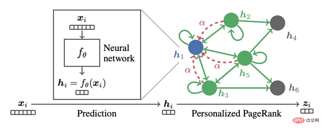
The same is such a model. If you use gradient descent to find it, and set The step size is b, and the iteration term is the partial derivative of the objective function at time k-1 with respect to Z.

when

When you can get:

##This is the APPNP model. The background of the emergence of the APPNP model is that the inverse operation of the matrix in the PPNP model is too complicated, and APPNP uses iterative approximation to solve it. It can also be understood that APPNP can converge to PPNP because both come from the same framework.

4. New GNN framework
As long as we design a new fitting term O##fit, and Design a corresponding graph regular term Oreg, and add a new solution process to get a new GNN model.
① Example 1: From all-pass filtering to low-pass filteringAs mentioned before, all-pass filtering Convolution kernel under the device F1##=F2=I , when the convolution kernel is the Laplacian matrix L It is a high pass filter. If the GNN obtained by weighting these two situations can encode low-pass information:

can get the exact solution:

## Similarly, we can solve it iteratively:

The regular term mentioned in the previous unified framework is equivalent to the L2 regular, which is equivalent to the difference information between any two points on the calculation graph. Some researchers feel that L2 regularization is too global and will cause the smoothness of the entire graph to tend to be the same, which is not entirely consistent with reality. Therefore, it was proposed to add an L1 regular term. The L1 regular term would penalize relatively large changes in the graph.


- We can use a more macro perspective to understand GNN
- We can start from this unified framework to design new GNN
2. Relational GNN model
1, RGCN
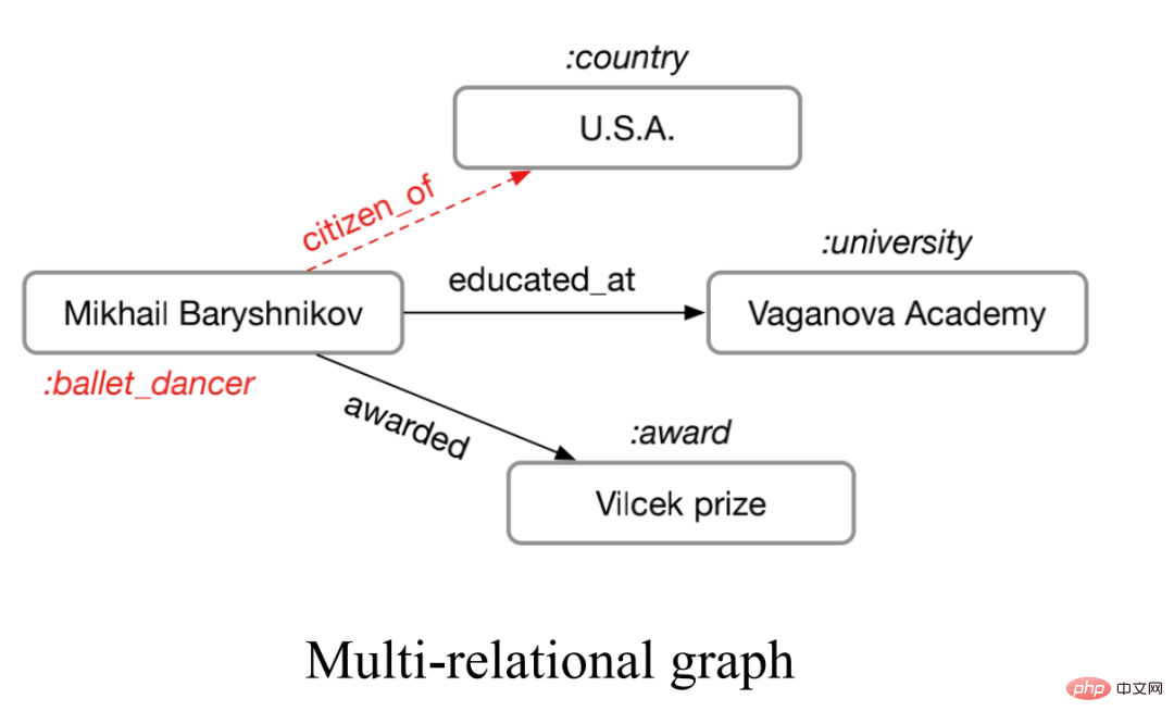
## The so-called multi-relationship graph refers to a graph with an edge type greater than 1, as shown in the figure below.
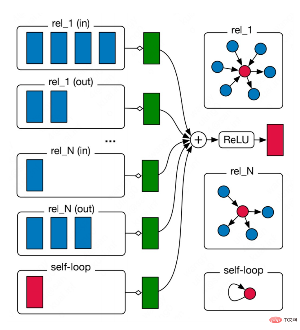

Nr are aggregated, among which Wr is the weight used to weight various relationships. Therefore, it can be seen that as the number of relationships in the graph increases, the weight matrix Wr will also increase, which will lead to the problem of over-parameterization ( Over-parameterization). In addition, splitting the topological relationship diagram according to relationships can also lead to over-smoothing. #In order to solve the problem of over-parameterization, CompGCN uses a vectorized relation encoder to replace N relations Matrix: The encoder contains relationships in three directions: forward, reverse, and self-loop: 2, CompGCN


Every iteration will also update the embedding of the relation.

But this heuristic design and such a parametric encoder are also Will cause excessive parameterization. Then, based on the above considerations, we get the starting point of our work: Can we design a more reliable GNN from the perspective of optimization goals, and at the same time solve the problems of existing GNNs.
3. Integrated Multi-Relationship Graph Neural Network
Our EMR GNN was published this year. Next, we will mainly focus on Three aspects are discussed on how we design a GCN suitable for multi-relationship graphs:
- How to design a suitable integrated optimization algorithm
- Message delivery mechanism
- How the GNN model is designed
1. Integrated optimization algorithm
This optimization algorithm needs to meet two requirements:
- Be able to capture multiple relationships on the graph at the same time
- Be able to model the importance of different relationships on the graph
The integrated multi-relationship graph regular term we propose on the multi-relationship graph is as follows:
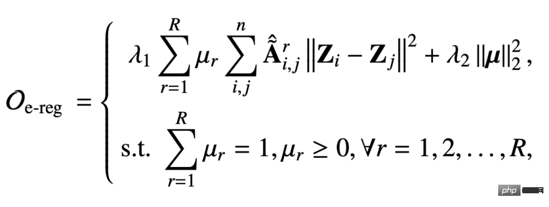
This regular term is also to capture the smoothing ability of the graph signal, but this adjacency matrix is captured under the relationship r and is subject to normalization Constrained parameters μr is to model the importance of a certain relationship. The second term is the second normal form regularization of the coefficient vector, which is to make the coefficient vector more uniform.
#In order to solve the problem of over-smoothing, we added a fitting term to ensure that the original feature information is not lost. The sum of the fitting term and the regular term is:
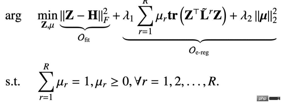
and what was mentioned in the previous chapter Compared with the unified framework, the objective function we design here includes two variables: node correction Z and relationship matrix parameter μ. So it is also a challenge to derive a message propagation mechanism based on such an optimization goal.
2. Derivation of message passing mechanism
Here we adopt an iterative optimization strategy:
- First fix the node representation Z, and then optimize the parameter μ
- Then optimize the node based on the result μ of the previous iteration Represent Z
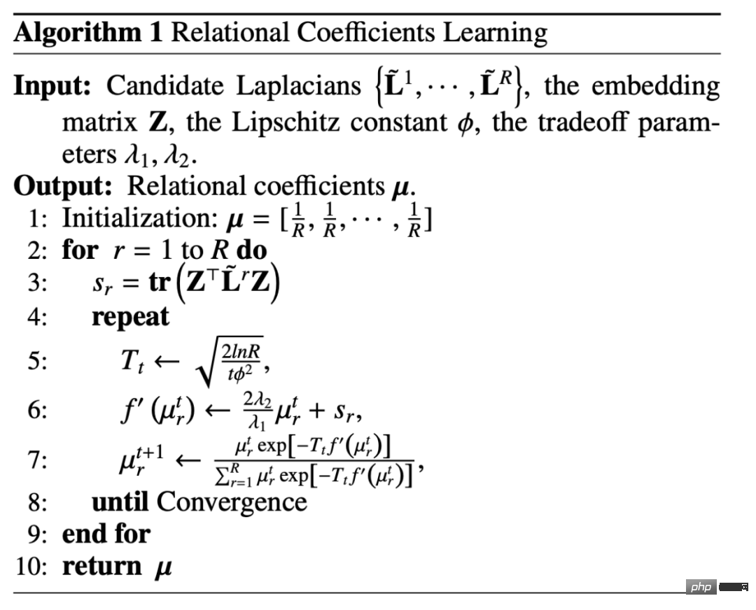
When the fixed node represents Z, the entire optimization objective degenerates into an objective function only related to μ, but this is a band Constrained objective function:
##This is actually a simplex constraint (constraint in a standard A convex function of μ on simplex). For this type of problem, we can use the Mirror Entropic Descent Algorithm to solve it. We will first find a constant, and then update the weight coefficient under each relationship. The entire update process is similar to the exponential gradient descent algorithm.
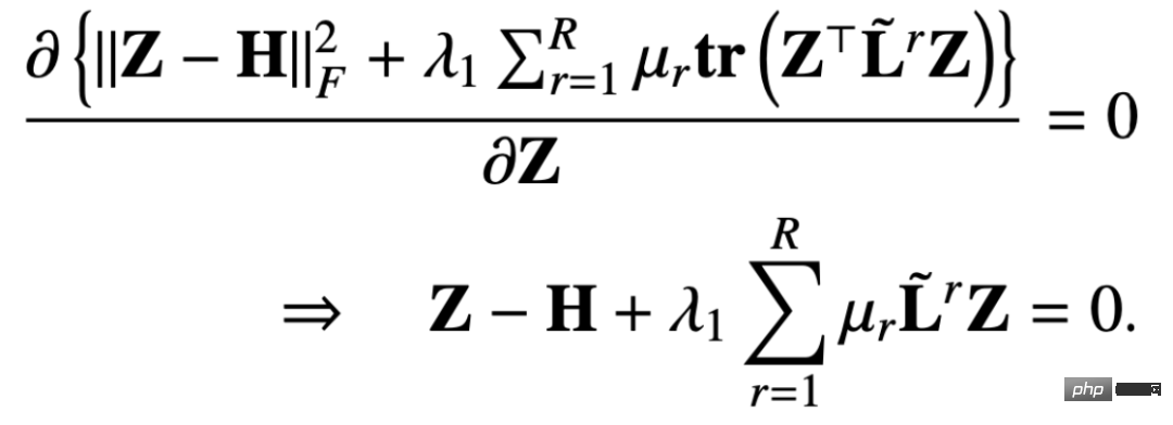
Fixed the relationship coefficient μ to update Z, then the optimization goal degenerates into the following This form:

In this way we find the partial derivative of the objective function with respect to Z, and let If the partial derivative is equal to 0, we can get:
##Then the closed-form solution of Z is:
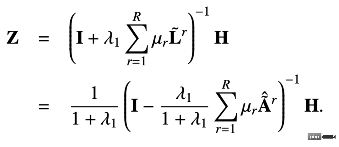
Similarly, we can use iteration to get an approximate solution. This process can be expressed as follows :

From the derived message passing mechanism we can prove that the design can avoid excessive Smooth and avoid over-parameterization. Below we can look at the proof process.
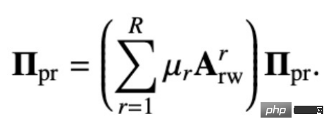
The original multi-relationship PageRank matrix is defined as follows:
The personalized multi-relationship PageRank matrix adds a probability of returning its own node on this basis:

By solving the above circular equation, you can get the multi-relationship personalized PageRank matrix:

Let us:
You can get:
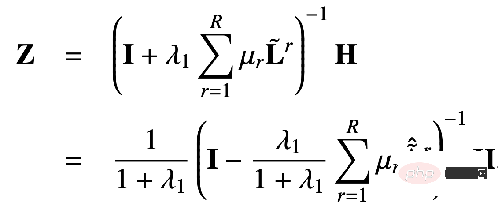
##this That is the closed-form solution obtained by our proposed solution. That is to say, our propagation mechanism can be equivalent to propagating feature H on the personalized PageRank matrix of the node. Because in this propagation mechanism, a node can return to its own node with a certain probability, which means that its own information will not be lost during the information transmission process, thereby preventing the problem of over-smoothing.
In addition, our model also alleviates the phenomenon of over-parameterization, because as can be seen from the formula, for each relationship our model only has A learnable coefficient μr , Compared with the number of parameters of the previous encoder or weight matrix w#r, the magnitude of our parameters is almost negligible. The following figure is the model architecture we designed:
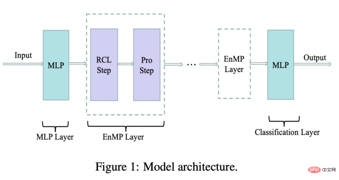
where RCL is the parameter learning step, and the Pro step is the feature propagation step. These two steps together form our messaging layer. So how do we integrate our messaging layer into the DNN without introducing more additional parameters? We also follow the decoupling design idea: first use an MLP to extract input features, and then pass through multiple layers of message passing layers we designed. Superimposing multiple layers will not lead to over-smoothing. The final transfer result is processed by MLP to complete node classification and can be used for downstream tasks. Use the formula to express the above process as follows:

##f(X;W) means that The input features are extracted through MLP, and the following EnMP(K) means that the extraction results are passed through the K layer message, gθ represents a classified MLP.
In back propagation we only need to update the parameters in the two MLPs, while the parameters in our EnMP are learned during the forward propagation process Yes, there is no need to update any parameters of EnMP during the backward propagation process.
We can compare the parameters of different mechanisms. We can see that the parameters of our EMR-GNN mainly come from the two MLPs before and after, and the relation coefficient. When the number of layers is greater than 3, we can know that the number of parameters of EMR-GNN is less than that of GCN, and even less than other heterogeneous graphs.

With such a small number of parameters, our EMR-GNN operates at different nodes as follows: The best level can still be achieved under classification tasks.

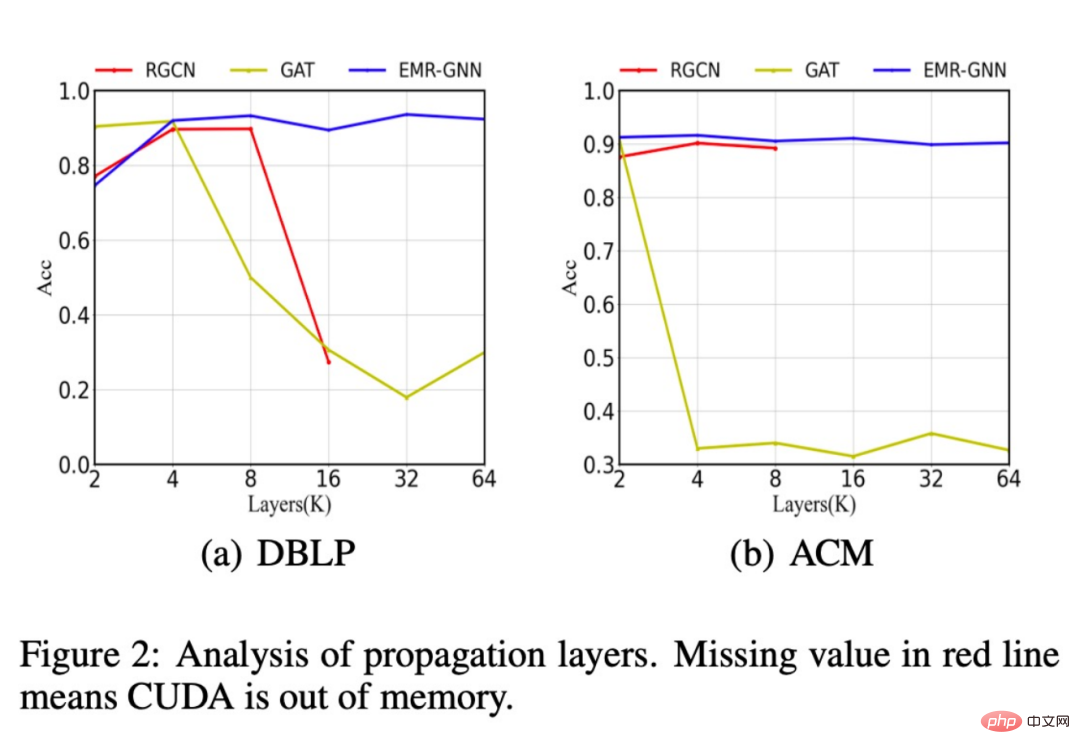
In addition, we also compared the changes in classification accuracy of different network structures after the number of layers increased. As shown in the figure below, when the number of layers increased to 64, our model can still maintain a high level Accuracy, while the original RGCN will encounter insufficient memory when the number of layers increases to more than 16 layers, and it is impossible to superimpose more layers. This is due to too many parameters. The performance of the GAT model is degraded due to over-smoothing.
In addition, we also found that our EMR-GNN performed better under smaller data sizes. It can achieve the classification accuracy of the whole sample, while RGCN drops a lot.
We also analyzed whether the relationship coefficient μr learned by EMR-GNN is really meaningful, so what is meaningful? We hope that the relationship coefficient μr relationship coefficient Give more weight to important relationships and less weight to unimportant relationships. The results of our analysis are shown in the figure below:
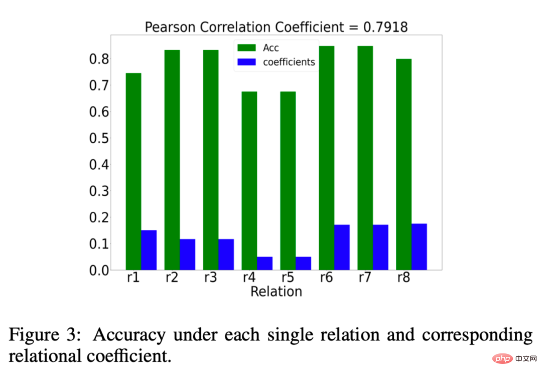
##The green histogram represents a The effect of classification under a certain relationship. If the classification accuracy is higher under a certain relationship, we can think that the relationship is important. The blue columns represent the relationship coefficients learned by our EMR-GNN. From the blue-green comparison, we can see that our relationship coefficient can reflect the importance of the relationship.
Finally we also made a visual display as shown below:

You can see that the node embedding trained by EMR-GNN can carry the structured information of the node, which can make the nodes of the same type more cohesive and different types as much as possible. Separate, the segmentation boundary is clearer than other networks.
##4. Summary1. We use a unified perspective to understand GNN
① From this perspective, we can easily see what problems there are with existing GNN
②This unified perspective can give us a way to redesign GNN Basics
#2. We try to design a new multi-relationship GNN from the perspective of the objective function## ① We First, an integrated optimization framework was designed
## ② Based on such an optimization framework, we derived a message passing mechanism
③ This message passing mechanism with a small number of parameters is simply combined with MLP to get EMR-GNN
3. EMR-GNN has What are the benefits?
## ① It relies on a reliable optimization goal, so the results obtained are credible, and its underlying principles can be explained mathematically
② It can solve the over-smoothing problem of the existing Relation GNN
## ③ Solve the over-parameterization problem
④ Easy to train, better results can be obtained with smaller parameter quantities
5. Q&A session
Q1: Is there any difference between the learning of relationship coefficients and the attention mechanism?
A1: The relationship coefficient learning here is an update process derived through the optimization framework, and attention is a process that needs to be learned based on backpropagation, so in terms of optimization, both There is a fundamental difference.
#Q2: How applicable is the model on large-scale data sets?
A2: We analyzed the complexity of the model in the appendix. In terms of complexity, we are on the same level as RGCN, but the number of parameters will be smaller than RGCN. , so our model is even more suitable for large-scale data sets.
#Q3: Can this framework incorporate edge information?
#A3: Can be integrated into the fitting term or regular term.
#Q4: Where should I learn these mathematical basics?
#A4: Part of it is based on previous work, and the other part of the mathematical theory related to optimization is also based on some classic optimization papers.
#Q5: What is the difference between a relationship diagram and a heterogeneous diagram?
#A5: The relationship graph is a heterogeneous graph, but we usually think of heterogeneous graphs as those whose node types or edge types are greater than 1. In the relationship diagram, we are particularly concerned about the relationship category greater than 1. It can be understood that the latter includes the former.
Q6: Can mini-batch training be supported?
A6: Supported.
Q7: Is the future research direction of GNN more inclined to strict, interpretable mathematical derivation rather than heuristic design?
#A7: We ourselves feel that strict interpretable mathematical derivation is a reliable design method.
The above is the detailed content of Integrated multi-graph neural network. For more information, please follow other related articles on the PHP Chinese website!

Hot AI Tools

Undresser.AI Undress
AI-powered app for creating realistic nude photos

AI Clothes Remover
Online AI tool for removing clothes from photos.

Undress AI Tool
Undress images for free

Clothoff.io
AI clothes remover

Video Face Swap
Swap faces in any video effortlessly with our completely free AI face swap tool!

Hot Article

Hot Tools

Notepad++7.3.1
Easy-to-use and free code editor

SublimeText3 Chinese version
Chinese version, very easy to use

Zend Studio 13.0.1
Powerful PHP integrated development environment

Dreamweaver CS6
Visual web development tools

SublimeText3 Mac version
God-level code editing software (SublimeText3)

Hot Topics
 1387
1387
 52
52
 Top 5 GenAI Launches of February 2025: GPT-4.5, Grok-3 & More!
Mar 22, 2025 am 10:58 AM
February 2025 has been yet another game-changing month for generative AI, bringing us some of the most anticipated model upgrades and groundbreaking new features. From xAI’s Grok 3 and Anthropic’s Claude 3.7 Sonnet, to OpenAI’s G
 How to Use YOLO v12 for Object Detection?
Mar 22, 2025 am 11:07 AM
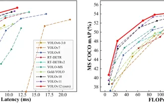
YOLO (You Only Look Once) has been a leading real-time object detection framework, with each iteration improving upon the previous versions. The latest version YOLO v12 introduces advancements that significantly enhance accuracy
 Best AI Art Generators (Free & Paid) for Creative Projects
Apr 02, 2025 pm 06:10 PM
The article reviews top AI art generators, discussing their features, suitability for creative projects, and value. It highlights Midjourney as the best value for professionals and recommends DALL-E 2 for high-quality, customizable art.
 Is ChatGPT 4 O available?
Mar 28, 2025 pm 05:29 PM
ChatGPT 4 is currently available and widely used, demonstrating significant improvements in understanding context and generating coherent responses compared to its predecessors like ChatGPT 3.5. Future developments may include more personalized interactions and real-time data processing capabilities, further enhancing its potential for various applications.
 Best AI Chatbots Compared (ChatGPT, Gemini, Claude & More)
Apr 02, 2025 pm 06:09 PM
The article compares top AI chatbots like ChatGPT, Gemini, and Claude, focusing on their unique features, customization options, and performance in natural language processing and reliability.
 How to Use Mistral OCR for Your Next RAG Model
Mar 21, 2025 am 11:11 AM
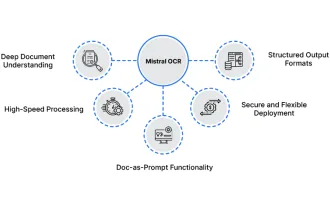
Mistral OCR: Revolutionizing Retrieval-Augmented Generation with Multimodal Document Understanding Retrieval-Augmented Generation (RAG) systems have significantly advanced AI capabilities, enabling access to vast data stores for more informed respons
 Top AI Writing Assistants to Boost Your Content Creation
Apr 02, 2025 pm 06:11 PM
The article discusses top AI writing assistants like Grammarly, Jasper, Copy.ai, Writesonic, and Rytr, focusing on their unique features for content creation. It argues that Jasper excels in SEO optimization, while AI tools help maintain tone consist
 Getting Started With Meta Llama 3.2 - Analytics Vidhya
Apr 11, 2025 pm 12:04 PM
Meta's Llama 3.2: A Leap Forward in Multimodal and Mobile AI Meta recently unveiled Llama 3.2, a significant advancement in AI featuring powerful vision capabilities and lightweight text models optimized for mobile devices. Building on the success o


