 Technology peripherals
 AI
AI
 An article discussing the issues and challenges in autonomous driving decision planning
An article discussing the issues and challenges in autonomous driving decision planning
In the positioning, perception, prediction, decision planning and control modules of autonomous driving, the perception module is like human eyes and ears, responsible for sensing the external environment; the control module is like human hands and feet. It is responsible for the final acceleration, deceleration, steering and other operations; the decision-making planning module is like the human brain, making behavioral decisions and trajectory generation based on the received perception and other information.
Welcome to follow the "Smart Driving Frontier" WeChat video account. Just like the human brain is divided into the left brain and the right brain, the decision-making planning module can be further divided into the behavioral decision-making layer (Behavioral Layer) and the motion planning layer. (Motion Planning).
After receiving the global path, the behavioral decision-making layer combines the sensory information to make specific behavioral decisions; the motion planning layer plans to generate a trajectory that satisfies specific constraints based on the specific behavioral decisions. This trajectory is as Inputs from the control module determine the vehicle's final travel path.
As the level of autonomous driving continues to improve, the importance of the decision-making and planning layer as the brain of autonomous driving has also increased. But compared with the human brain, the brain of autonomous driving still has a long way to catch up. This article will detail the problems and challenges of Motion Planning in path planning through ten thousand words.
01 Commonly used algorithms for Motion Planning
The Motion Planning algorithm was developed from the field of robotics, and has gradually developed various algorithms suitable for the field of autonomous driving. The paper [1] provides an overview of the trajectory generation method of Motion Planning. The introduced method is shown in the figure below.
Algorithms based on sampling search: Dijkstra, RRT, A*, hybridA* and Lattice, etc.;
Algorithms based on curve interpolation: RS curve, Dubins curve, polynomial curve, Bezier curve and spline curves, etc.;
Optimization-based algorithms: Apollo’s piecewise-jerk, etc.;
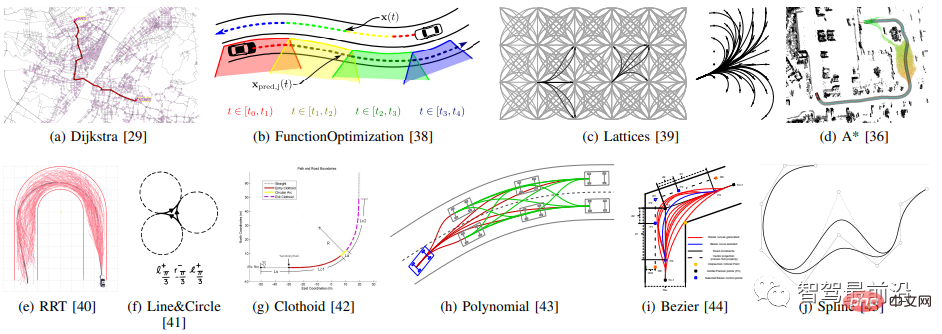
The above algorithms are generally used in combination with each other of. For example, polynomial curves need to sample terminal states, Bezier curves need to sample control points, and hybird A* uses RS curves or Dubins curves, etc.
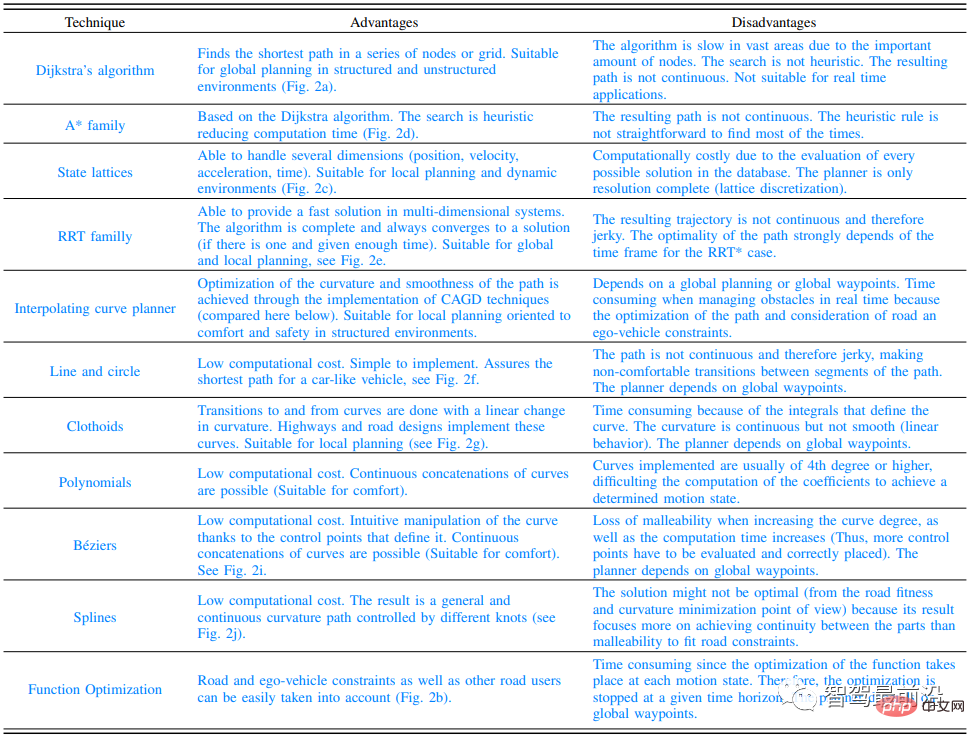
The paper [1] summarizes the advantages and disadvantages of various trajectory generation algorithms, as shown in the figure below. It can be seen that no algorithm is perfect, and an appropriate algorithm needs to be selected based on specific scenarios and working conditions. Currently, polynomial curve interpolation (high-speed scenarios) and optimization algorithms are widely used in the industry.
02 Motion Planning issues and challenges
The Motion Planning algorithm introduced above can basically solve most of the trajectory generation problems in autonomous driving scenarios. Trajectory generation Algorithms are no longer the main bottleneck. However, there are still many challenges that need to be overcome in the field of Motion Planning, mainly including the following aspects:
Optimality problem;
Cognitive reasoning problem;
Uncertainty/Probability;
Single-Agent;
Multiple-Agent;
Engineering issues.
2.1 Optimality problem
Global optimization is an NP-hard problem [3]. For real-time performance, most of the industry adopts horizontal and vertical decoupling planning methods. However, doing so will sacrifice optimality, and good vehicle behavior cannot be obtained under some working conditions, such as overtaking [2], oncoming vehicles, centripetal acceleration constraint processing, and horizontal planning that requires consideration of longitudinal planning capabilities.
For example, when there is a decelerating vehicle in front of the Autonomous Driving Car (ADC), the horizontal and vertical decoupling method generally only overtakes when the speed of the vehicle in front reduces to a certain value. . The behavior of ADC is to first slow down or even stop, and then drive around obstacles. This is obviously not the optimal driving strategy.
If a spatio-temporal integrated planning method is adopted, deceleration or parking behaviors can be avoided. The left picture in the figure below is an example of the decoupling method. When there is a decelerating and parking vehicle ahead, the ADC will decelerate. The picture on the right is an example of spatio-temporal planning. ADC will overtake when the vehicle in front slows down.

2.2 Cognitive reasoning problem
2.2.1 Map topology reasoning
Take Apollo as an example, PNC The Map module extracts data from the HD Map module to form a reference line, and queries road elements through the API interface of the HD Map module. However, the Motion Planning module ignores some road topological relationships, such as incoming and outgoing intersections, and these special road topologies will affect vehicle behavior.
In addition, if there is no HD Map module and relies solely on visual lane lines, abnormal lane line perception will occur at this time. The road topology problem is particularly prominent in the incoming and outgoing roads and intersection roads.
2.2.2 Unified modeling of obstacles
Participants in the traffic scene include vehicles, motorcycles, bicycles, pedestrians, cones, etc. Broadly speaking, it also includes static map elements such as crosswalks, traffic lights, and road speed limits. Motion Planning needs to make different decisions for different elements. Unified modeling of obstacles can simplify the problem and improve computational efficiency.

2.2.3 Scenario Cognitive Reasoning
Due to the complexity of the real environment, it is difficult for one decision-making strategy or planning method to handle different working conditions. Therefore, classifying the driving environment and choosing different strategies in different scenarios can improve the performance of Motion Planning. So how to carry out scene classification and scene recognition, and what are the differences between Motion Planning in different scenes? These problems all need to be solved. The scene classification in Aopllo is LANE_FOLLOW, SIDE_PASS, STOP_SIGN_UNPROTECTED, etc. There are two methods of scene recognition, one is through rules and the other is through machine learning. Different scenarios have different stages, and tasks are executed in sequence in the stages. Even the same task may have different parameter configurations in different scenarios. Based on the characteristics of urban scenes with many intersections, congestion and lane changes, Haimou divides driving scenes into ten categories, which is obviously different from the scenario classification in Apollo. However, Haimou's scene recognition method cannot And know. Hao Mo also proposed the concept of driving environment entropy to describe the congestion state of the driving environment. 2.3 Uncertainty2.3.1 Positioning Uncertainty
In most Motion Planning, the positioning is considered to be accurate enough. However, in actual scenes, positioning is often inaccurate due to problems such as occlusion and multipath interference. As shown in the lower left figure in the paper [6], the positioning error causes errors in the road boundary queried from the HD Map module, so that the planning and vehicle driving trajectories are on the road boundary. PictureThe paper assumes that positioning uncertainty is a Gaussian distribution, and the positioning module can calculate the expectation and variance of the probability distribution. The paper converts the vehicle coordinate system to the UTM coordinate system. According to the high-speed distribution of positioning and the coordinate transformation formula, the uncertainty of the vehicle's surrounding environment under the influence of positioning can be calculated, as shown in the figure on the right above, where the darker the color. The greater the uncertainty, the uncertainty calculation formula is mainly obtained by the following formula. It can be found that the farther away from the ADC, the higher the uncertainty. As the vehicle moves forward, its uncertainty will be updated. The path planning method uses the Lattice (quintic polynomial curve) method, and two items are added during cost calculation. One is a hard constraint: the maximum uncertainty of a point on the planning path cannot be greater than a certain threshold; the second is to add the weight sum of uncertainties in the cost function.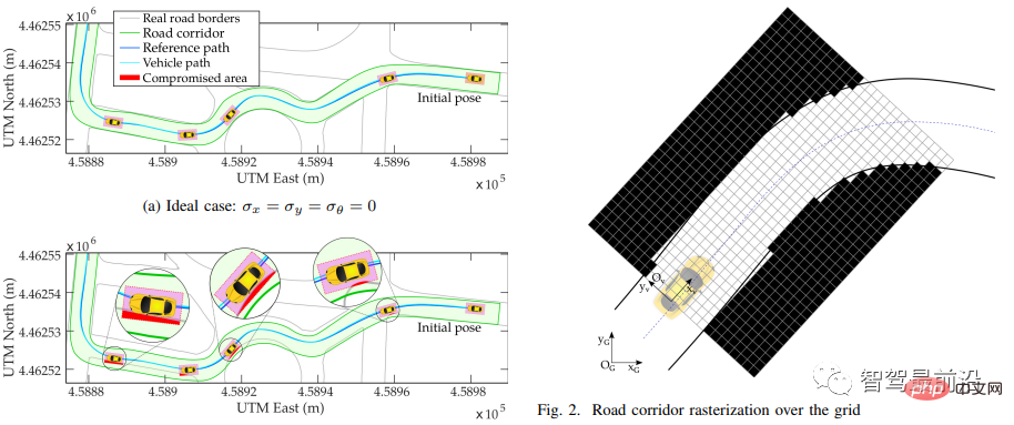
2.3.2 Perception uncertainty
Due to sensor noise, vehicle vibration, driving environment and imperfect algorithms, perception The results obtained are uncertain or even wrong. Perceived uncertainty can cause insecurity in Motion Planning results. A simple processing method is to add a buffer, but a rough processing method will reduce the feasible range of Motion Planning and may result in an overly aggressive or overly conservative driving strategy. The paper [7] takes the parking application equipped with Around View Monitoring (AVM) as an example. Due to the perception error, the path planning will cause parking at the actual overtaking position, and a collision may occur, as shown in the left figure below. The paper models the perceived uncertainty as a Gaussian distribution. The farther the perceived effect is from the ADC, the higher the uncertainty, as shown in the right figure below.
Parking space sampling: Sampling the two closest corner points to the ADC, treating the sampling points as normally distributed, and calculating the parking center of the ADC rear axle based on the sampling corner points and the length of the set parking space. point;
Path candidate generation: Use ocp theory to perform path planning for each sampling point, in which the time domain problem is converted into the Ferent coordinate system, and SQP is used to solve the nonlinear problem;
Optimal Path Selection: Use utility theory to select the optimal path. Utility function is: EU(s) = P(s) x Uideal(s) (1-P(s)) x Ureal(s), where P(s) is the probability of the path corresponding to the sampling point, and Uideal is the path to the target. The deviation utility function value of the point (sensingly detected at the current moment, not obtained by sampling), Ureal is the utility function value on the path to the current position of the ADC.

2.3.3 Prediction Uncertainty
Prediction is an important part of realizing high-level autonomous driving above L4. However, as of now, forecasting remains a very difficult problem for the entire industry. Therefore, the accuracy of prediction is very poor, and it is very important to do motion planning under the uncertainty of prediction results.
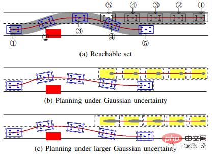
The paper [8] proposes a planning architecture based on Gaussian distribution to deal with the problem of unsafe planning trajectories caused by uncertainty in prediction and control.
Candidate trajectory generation: generated through multi-stage horizontal and vertical sampling. It can be understood as the Aopllo Lattice method.
Predicted trajectory generation: When predicting (planning) the trajectory of a certain vehicle, it is considered that other vehicles are traveling at a constant speed and their states are determined. Then, by calculating the cost of the candidate trajectory, we get optimal predicted trajectory. The probability distribution of the predicted trajectory is then calculated through Kalman filtering, assuming that it follows a normal distribution.
ADC trajectory generation: At this time, the uncertainty of the predictions of other traffic participants needs to be considered. For each candidate trajectory, the control error is calculated through the LQR algorithm, and then the probability distribution of the trajectory is calculated through Kalman filtering. When cos calculation is performed for trajectory evaluation, collision detection is based on the probability distribution of the predicted and ADC planning trajectories, that is Collisions cannot occur within any probability distribution.
The author believes that this method is equivalent to adding an adaptive buffer to the box, while a conventional fixed-size buffer will lead to conservative or aggressive driving behavior.
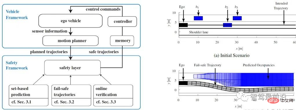
Paper [9] The paper proposes a fail-safe mechanism that can be embedded in the existing Motion Planning framework, which is divided into three parts:
Set- based prediction: Based on the developed driving strategies and vehicle kinematics models of traffic participants, the original single predicted trajectory of traffic participants is changed to multiple predicted trajectories;
Fail-safe trajectory: Based on the predicted As a result, the first trajectory point with collision risk in the original planning trajectory is calculated, and then the trajectory is generated based on the optimization theory;
Online verification: Project the ADC on the trajectory generated in the second step to determine whether it is And the first step is to predict whether there is a collision in the vehicle trajectory.
I feel that this method is a re-doing of Motion Planning. Since the paper does not describe whether the fail-safe trajectory considers the decision results, it may cause the safe trajectory not to satisfy the decision results, and this paper is only a simulation, and Has no practical application.
2.3.4 Partially Observable Environments
Due to the limited sensing range of the sensor itself and the uncertainty of the sensing results, in It will be further amplified in bad lighting or bad weather. In urban working conditions, the occlusion of buildings will cause incomplete perception, as shown in the figure below. In addition, large vehicles can also cause perceptual occlusion problems, and most Motion Planning is processed with complete perception, so the planning results are very unsafe.
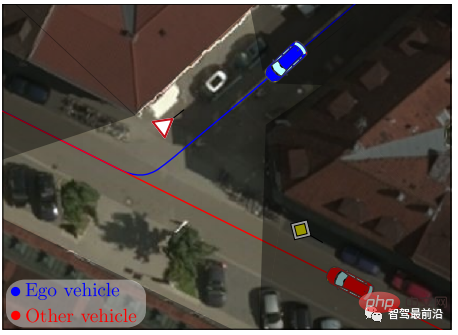
The paper [10] proposes a motion planning that handles incomplete perception of safety, so that the planned trajectory can be safe under the maximum braking capacity of the vehicle in the most dangerous situations. Park your car without crashing. It is divided into two situations: one is when driving on a straight road, considering the uncertainty of perception and the range of perception distance, and the second is when driving at an urban intersection, where incomplete perception is considered. And it is easy to embed into other Motion Planning architectures. The author conducted simulation verification in the trajectory planning based on the optimization method previously proposed (Figure (b) in the review).
The author designed several assumptions for his theory:
The longitudinal position and velocity information of positioning follows Gaussian distribution;
The effective range of perception is known, and the perception The result follows Gaussian distribution;
The map information contains the location of the building and is a convex polygon;
Use Intelligent Driver Model (IDM) for vehicle acceleration prediction.
Since the paper deals with two situations: straight roads and intersections, scene recognition is required. The paper uses a rule-based approach for scene recognition.

The upper left picture: the red dotted line is the time when the observed environment is sensed, and the black dotted line is the time for Motion Planning. It can be seen that the sensing information used by Motion Planning is before the tp time of. In addition, because Motion Planning must ensure continuity, the planned trajectory within the Motion Planning calculation cycle tpin must be consistent. More importantly, due to the delay of the actuator, the safety of the trajectory must be ensured within the tsafe time. In the paper, tsafe= 2tpin;
Top and middle picture: Driving on a straight road is divided into two situations: there are no vehicles within the sensing range or there are vehicles within the sensing range: First, there are no vehicles within the sensing range, assuming there are vehicles outside the driving sensing range A stationary vehicle is set as a virtual stationary obstacle. Through its Gaussian distribution characteristics, it can be calculated to satisfy the longitudinal displacement and speed constraints of braking with the maximum braking capacity within the tsafe moment; secondly, if there is a vehicle within the sensing range, consider that the sensing is not possible. The most dangerous situation under deterministic conditions, that is, the vehicle in front is braking with the maximum braking capacity. Through its Gaussian distribution characteristics, it can be calculated to satisfy the longitudinal displacement and speed constraints of braking with the maximum braking capacity within the tsafe time;
Above right picture: Driving at an intersection, according to the IDM model, it is calculated whether the ADC needs to give way or has the right of way and needs to clearly indicate its intention to pass first. Finally converted to two types of constraints for straight driving.
2.4 Single Agent
Single Agent considers it a single agent problem, that is, the ADC will make decisions about the surrounding environment without considering the impact of the ADC's behavioral decisions on other traffic participants. Obviously this This assumption is incorrect, but it simplifies the Motion Planning problem.
Behavioral decision-making is another important aspect that affects the development of autonomous driving. As the level of autonomous driving increases, the importance of behavioral decision-making becomes higher. The difficulty in behavioral decision-making is how to embody the intelligence of autonomous vehicles and how to enable autonomous vehicles to handle high-dimensional, multi-constraint complex scenarios like human drivers, or even perform better than human drivers.
Most current methods are rule-based methods with limited capabilities. In terms of behavioral decision-making based on the rule method, in off-ramp conditions, a distance threshold from the ramp entrance is generally designed. When the distance from the ADC to the ramp is within the threshold, the lane change to the rightmost lane begins.
Assuming that this threshold is 2km, if the ADC is driving in the middle lane at 2.1m of the ramp intersection, and there is a car in front at a low speed, the rule-based behavioral decision-making will generally choose to change to the left lane. (the left lane has a high speed limit, and overtaking must follow the left lane. It can be seen from Xiaopeng NGP and others that the left lane has priority). However, the distance threshold to the ramp entrance after changing lanes is less than 2km. At this time, it is necessary to change lanes to the rightmost lane, and it is necessary to perform two consecutive lane changes, which will appear not smart enough.
Another example is driving in the rightmost lane 500m before the ramp. If the road ahead cannot be driven due to construction or an accident, the driver can only take over. It can be seen that due to the complexity of real-life working conditions, it is difficult to achieve a good driving experience with a rule-based behavioral decision-making method.
Hong Kong University of Science and Technology's behavioral decision-making work on OPMDP [11] has a certain improvement in performance compared to the rule-based method. It prunes the behavior of ADC and other traffic participants, reducing the OPMDP time consuming. However, it takes into account that other traffic participants will avoid the ADC's behavior, etc. It can be seen that it is a Multiple Agent problem to deal with.
2.5 Multiple Agent
In the above-mentioned Single Agent, it is believed that traffic participants will not make corresponding decisions on the behavior of the ADC. But in reality, when the ADC makes After the decision is made, its behavior will affect the behavior of other traffic participants, reducing the credibility of the original prediction results. In particular, some simple rule-based predictions do not depend on the Motion Planning results, or use the previous frame of Motion Planning. The result (Apollo).
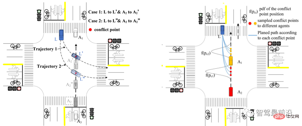
For example, in the left picture below, when ADC L is traveling along trajectory 1, A2 may slow down to avoid it. As ADC L travels along trajectory 2, A2 may accelerate through the intersection. But when ADC L is driving along trajectory 2, it is predicted that A2 may accelerate through the intersection, but A2 may misunderstand ADC L's intention and slow down, causing the two vehicles to lock up. Therefore, how ADC understands the intentions of other traffic participants and how other traffic vehicles understand the intentions of ADC is crucial [12].
2.6 Engineering issues
We also face some engineering issues in Motion Planning, mainly including the following aspects.
Real-time: The optimality problem mentioned in the first question. If it is to be solved, due to the complexity of search calculations in three-dimensional space, its real-time performance can be guaranteed. This also limits the application of joint spatio-temporal planning. A reason. In addition, large-scale constraints and nonlinearity in the optimization algorithm also face real-time challenges.
Completeness: Algorithms such as interpolation and Lattice are probabilistically complete. Especially in complex multi-obstacle environments, it is difficult to obtain a collision-free trajectory with limited sampling. The optimization method cannot achieve completeness due to numerical solution, and the commonly used osqp solver may even give an incorrect solution.
Difficult to quantify: Most of the evaluation indicators in Motion Planning are subjective, such as comfort and passability, etc., which are difficult to quantitatively evaluate. Different engineers adjust the parameters to get different body sensations, which are also different from the subjective feelings of passengers. Therefore, machine learning methods are proposed to learn parameters or lane changing strategies in Motion Planning.
03 Industry Solutions
In response to the above problems and challenges, companies in the industry are also actively exploring and proposing some solutions, one or two of which are listed below.
Qingzhou Zhihang uses space-time joint planning to solve the optimality problem, improve planning performance, and develops a self-developed nonlinear planner for efficient solution [2].
In the new generation framework of TuSimple, the perception module provides uncertainty or probability information while providing information such as obstacle location and speed to ensure that decision-making planning can make safe and comfortable decisions in advance [13 ].
Tesla uses Planner for other vehicles used by traffic participants. However, when interacting with other vehicles, planning should not be just for the ADC, but should be planned jointly for all traffic participants and optimized for the traffic flow of the overall scene. To do this, the autopilot planner is run for each participating object in the scene. In addition, for parking scenarios, the A search algorithm and neural network combination strategy are used, which greatly reduces the node exploration of the A algorithm [15].
Xpeng and Tesla have optimized the problem of missing lane lines and changes in road topology [14].
Waymo proposed ChauffeurNet to improve decision-making performance [16], and Apollo proposed its own reinforcement learning architecture based on ChauffeurNet [17].
The above is the detailed content of An article discussing the issues and challenges in autonomous driving decision planning. For more information, please follow other related articles on the PHP Chinese website!

Hot AI Tools

Undresser.AI Undress
AI-powered app for creating realistic nude photos

AI Clothes Remover
Online AI tool for removing clothes from photos.

Undress AI Tool
Undress images for free

Clothoff.io
AI clothes remover

AI Hentai Generator
Generate AI Hentai for free.

Hot Article

Hot Tools

Notepad++7.3.1
Easy-to-use and free code editor

SublimeText3 Chinese version
Chinese version, very easy to use

Zend Studio 13.0.1
Powerful PHP integrated development environment

Dreamweaver CS6
Visual web development tools

SublimeText3 Mac version
God-level code editing software (SublimeText3)

Hot Topics
 Why is Gaussian Splatting so popular in autonomous driving that NeRF is starting to be abandoned?
Jan 17, 2024 pm 02:57 PM
Written above & the author’s personal understanding Three-dimensional Gaussiansplatting (3DGS) is a transformative technology that has emerged in the fields of explicit radiation fields and computer graphics in recent years. This innovative method is characterized by the use of millions of 3D Gaussians, which is very different from the neural radiation field (NeRF) method, which mainly uses an implicit coordinate-based model to map spatial coordinates to pixel values. With its explicit scene representation and differentiable rendering algorithms, 3DGS not only guarantees real-time rendering capabilities, but also introduces an unprecedented level of control and scene editing. This positions 3DGS as a potential game-changer for next-generation 3D reconstruction and representation. To this end, we provide a systematic overview of the latest developments and concerns in the field of 3DGS for the first time.
 How to solve the long tail problem in autonomous driving scenarios?
Jun 02, 2024 pm 02:44 PM
Yesterday during the interview, I was asked whether I had done any long-tail related questions, so I thought I would give a brief summary. The long-tail problem of autonomous driving refers to edge cases in autonomous vehicles, that is, possible scenarios with a low probability of occurrence. The perceived long-tail problem is one of the main reasons currently limiting the operational design domain of single-vehicle intelligent autonomous vehicles. The underlying architecture and most technical issues of autonomous driving have been solved, and the remaining 5% of long-tail problems have gradually become the key to restricting the development of autonomous driving. These problems include a variety of fragmented scenarios, extreme situations, and unpredictable human behavior. The "long tail" of edge scenarios in autonomous driving refers to edge cases in autonomous vehicles (AVs). Edge cases are possible scenarios with a low probability of occurrence. these rare events
 Choose camera or lidar? A recent review on achieving robust 3D object detection
Jan 26, 2024 am 11:18 AM
0.Written in front&& Personal understanding that autonomous driving systems rely on advanced perception, decision-making and control technologies, by using various sensors (such as cameras, lidar, radar, etc.) to perceive the surrounding environment, and using algorithms and models for real-time analysis and decision-making. This enables vehicles to recognize road signs, detect and track other vehicles, predict pedestrian behavior, etc., thereby safely operating and adapting to complex traffic environments. This technology is currently attracting widespread attention and is considered an important development area in the future of transportation. one. But what makes autonomous driving difficult is figuring out how to make the car understand what's going on around it. This requires that the three-dimensional object detection algorithm in the autonomous driving system can accurately perceive and describe objects in the surrounding environment, including their locations,
 Have you really mastered coordinate system conversion? Multi-sensor issues that are inseparable from autonomous driving
Oct 12, 2023 am 11:21 AM
The first pilot and key article mainly introduces several commonly used coordinate systems in autonomous driving technology, and how to complete the correlation and conversion between them, and finally build a unified environment model. The focus here is to understand the conversion from vehicle to camera rigid body (external parameters), camera to image conversion (internal parameters), and image to pixel unit conversion. The conversion from 3D to 2D will have corresponding distortion, translation, etc. Key points: The vehicle coordinate system and the camera body coordinate system need to be rewritten: the plane coordinate system and the pixel coordinate system. Difficulty: image distortion must be considered. Both de-distortion and distortion addition are compensated on the image plane. 2. Introduction There are four vision systems in total. Coordinate system: pixel plane coordinate system (u, v), image coordinate system (x, y), camera coordinate system () and world coordinate system (). There is a relationship between each coordinate system,
 This article is enough for you to read about autonomous driving and trajectory prediction!
Feb 28, 2024 pm 07:20 PM
Trajectory prediction plays an important role in autonomous driving. Autonomous driving trajectory prediction refers to predicting the future driving trajectory of the vehicle by analyzing various data during the vehicle's driving process. As the core module of autonomous driving, the quality of trajectory prediction is crucial to downstream planning control. The trajectory prediction task has a rich technology stack and requires familiarity with autonomous driving dynamic/static perception, high-precision maps, lane lines, neural network architecture (CNN&GNN&Transformer) skills, etc. It is very difficult to get started! Many fans hope to get started with trajectory prediction as soon as possible and avoid pitfalls. Today I will take stock of some common problems and introductory learning methods for trajectory prediction! Introductory related knowledge 1. Are the preview papers in order? A: Look at the survey first, p
 SIMPL: A simple and efficient multi-agent motion prediction benchmark for autonomous driving
Feb 20, 2024 am 11:48 AM
Original title: SIMPL: ASimpleandEfficientMulti-agentMotionPredictionBaselineforAutonomousDriving Paper link: https://arxiv.org/pdf/2402.02519.pdf Code link: https://github.com/HKUST-Aerial-Robotics/SIMPL Author unit: Hong Kong University of Science and Technology DJI Paper idea: This paper proposes a simple and efficient motion prediction baseline (SIMPL) for autonomous vehicles. Compared with traditional agent-cent
 nuScenes' latest SOTA | SparseAD: Sparse query helps efficient end-to-end autonomous driving!
Apr 17, 2024 pm 06:22 PM
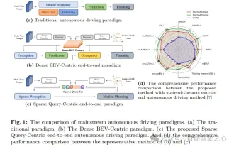
Written in front & starting point The end-to-end paradigm uses a unified framework to achieve multi-tasking in autonomous driving systems. Despite the simplicity and clarity of this paradigm, the performance of end-to-end autonomous driving methods on subtasks still lags far behind single-task methods. At the same time, the dense bird's-eye view (BEV) features widely used in previous end-to-end methods make it difficult to scale to more modalities or tasks. A sparse search-centric end-to-end autonomous driving paradigm (SparseAD) is proposed here, in which sparse search fully represents the entire driving scenario, including space, time, and tasks, without any dense BEV representation. Specifically, a unified sparse architecture is designed for task awareness including detection, tracking, and online mapping. In addition, heavy
 FisheyeDetNet: the first target detection algorithm based on fisheye camera
Apr 26, 2024 am 11:37 AM
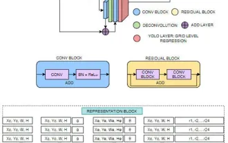
Target detection is a relatively mature problem in autonomous driving systems, among which pedestrian detection is one of the earliest algorithms to be deployed. Very comprehensive research has been carried out in most papers. However, distance perception using fisheye cameras for surround view is relatively less studied. Due to large radial distortion, standard bounding box representation is difficult to implement in fisheye cameras. To alleviate the above description, we explore extended bounding box, ellipse, and general polygon designs into polar/angular representations and define an instance segmentation mIOU metric to analyze these representations. The proposed model fisheyeDetNet with polygonal shape outperforms other models and simultaneously achieves 49.5% mAP on the Valeo fisheye camera dataset for autonomous driving


