

How to build a decision tree in Python

Decision Tree
Decision trees are an integral part of today's most powerful supervised learning methods. A decision tree is basically a flowchart of a binary tree where each node splits a set of observations based on some characteristic variable.
The goal of a decision tree is to divide data into groups so that every element in a group belongs to the same category. Decision trees can also be used to approximate continuous target variables. In this case, the tree will be split such that each group has the smallest mean squared error.
An important property of decision trees is that they are easily interpretable. You don't need to be familiar with machine learning techniques at all to understand what decision trees are doing. Decision tree diagrams are easy to interpret.
Pros and Cons
The advantages of the decision tree method are:
The decision tree can generate understandable rules.
Decision trees perform classification without requiring extensive calculations.
Decision trees can handle continuous variables and categorical variables.
Decision trees provide a clear indication of which fields are most important.
The disadvantages of the decision tree method are:
Decision trees are not suitable for estimation tasks where the goal is to predict continuous attribute values.
Decision trees are prone to errors in classification problems with many classes and few training samples.
Training of decision trees can be computationally expensive. The process of generating decision trees is computationally very expensive. At each node, each candidate split field must be sorted to find its best split. In some algorithms, using combinations of fields, the best combination of weights must be searched. Pruning algorithms can also be expensive because many candidate subtrees must be formed and compared.
Python Decision Tree
Python is a general-purpose programming language that provides data scientists with powerful machine learning packages and tools. In this article, we will use scikit-learn, the most famous machine learning package in Python, to build a decision tree model. We will create the model using the "DecisionTreeClassifier" algorithm provided by scikit learn and then visualize the model using the "plot_tree" function.
Step 1: Import package
The main software packages we use to build models are pandas, scikit learn and NumPy. Follow the code to import the required packages in python.
import pandas as pd # 数据处理 import numpy as np # 使用数组 import matplotlib.pyplot as plt # 可视化 from matplotlib import rcParams # 图大小 from termcolor import colored as cl # 文本自定义 from sklearn.tree import DecisionTreeClassifier as dtc # 树算法 from sklearn.model_selection import train_test_split # 拆分数据 from sklearn.metrics import accuracy_score # 模型准确度 from sklearn.tree import plot_tree # 树图 rcParams['figure.figsize'] = (25, 20)
After importing all the packages needed to build our model, it’s time to import the data and do some EDA on it.
Step 2: Import data and EDA
In this step we will use the "Pandas" package provided in python to import and do some EDA on it . We will build our decision tree model on a dataset that is a dataset of medications that are prescribed to patients based on specific criteria. Let’s import the data using python!
Python implementation:
df = pd.read_csv('drug.csv') df.drop('Unnamed: 0', axis = 1, inplace = True) print(cl(df.head(), attrs = ['bold']))Output:
Age Sex BP Cholesterol Na_to_K Drug 0 23 F HIGH HIGH 25.355 drugY 1 47 M LOW HIGH 13.093 drugC 2 47 M LOW HIGH 10.114 drugC 3 28 F NORMAL HIGH 7.798 drugX 4 61 F LOW HIGH 18.043 drugY
Now we have a clear idea of the dataset. After importing the data, let's use the "info" function to get some basic information about the data. Information provided by this function includes number of entries, index number, column name, non-null value count, attribute type, etc.
Python implementation:
df.info()
Output:
<class> RangeIndex: 200 entries, 0 to 199 Data columns (total 6 columns): # Column Non-Null Count Dtype --- ------ -------------- ----- 0 Age 200 non-null int64 1 Sex 200 non-null object 2 BP 200 non-null object 3 Cholesterol 200 non-null object 4 Na_to_K 200 non-null float64 5 Drug 200 non-null object dtypes: float64(1), int64(1), object(4) memory usage: 9.5+ KB</class>
Step 3: Data processing
We can See that attributes like Sex, BP and Cholesterol are categorical and object type in nature. The problem is that the decision tree algorithm in scikit-learn inherently does not support X variables (features) being of type "object". Therefore, it is necessary to convert these "object" values into "binary" values. Let us use python to implement
Python implementation:
for i in df.Sex.values: if i == 'M': df.Sex.replace(i, 0, inplace = True) else: df.Sex.replace(i, 1, inplace = True) for i in df.BP.values: if i == 'LOW': df.BP.replace(i, 0, inplace = True) elif i == 'NORMAL': df.BP.replace(i, 1, inplace = True) elif i == 'HIGH': df.BP.replace(i, 2, inplace = True) for i in df.Cholesterol.values: if i == 'LOW': df.Cholesterol.replace(i, 0, inplace = True) else: df.Cholesterol.replace(i, 1, inplace = True) print(cl(df, attrs = ['bold']))
Output:
Age Sex BP Cholesterol Na_to_K Drug 0 23 1 2 1 25.355 drugY 1 47 1 0 1 13.093 drugC 2 47 1 0 1 10.114 drugC 3 28 1 1 1 7.798 drugX 4 61 1 0 1 18.043 drugY .. ... ... .. ... ... ... 195 56 1 0 1 11.567 drugC 196 16 1 0 1 12.006 drugC 197 52 1 1 1 9.894 drugX 198 23 1 1 1 14.020 drugX 199 40 1 0 1 11.349 drugX [200 rows x 6 columns]
We can observe that all "object" values are processed into "binary" values to represent categorical data. For example, in the cholesterol attribute, values showing "low" are processed as 0, and "high" values are processed as 1. Now we are ready to create the dependent and independent variables from the data.
Step 4: Split the Data
After processing our data into the correct structure, we now set the "X" variable (independent variable), "Y "Variable (dependent variable). Let us use python to implement
Python implementation:
X_var = df[['Sex', 'BP', 'Age', 'Cholesterol', 'Na_to_K']].values # 自变量 y_var = df['Drug'].values # 因变量 print(cl('X variable samples : {}'.format(X_var[:5]), attrs = ['bold'])) print(cl('Y variable samples : {}'.format(y_var[:5]), attrs = ['bold']))Output:
X variable samples : [[ 1. 2. 23. 1. 25.355] [ 1. 0. 47. 1. 13.093] [ 1. 0. 47. 1. 10.114] [ 1. 1. 28. 1. 7.798] [ 1. 0. 61. 1. 18.043]] Y variable samples : ['drugY' 'drugC' 'drugC' 'drugX' 'drugY']
We can now use the "train_test_split" algorithm in scikit learn to The data is split into a training set and a test set, which contain the X and Y variables we defined. Follow the code to split data in python.
Python implementation:
X_train, X_test, y_train, y_test = train_test_split(X_var, y_var, test_size = 0.2, random_state = 0) print(cl('X_train shape : {}'.format(X_train.shape), attrs = ['bold'], color = 'black')) print(cl('X_test shape : {}'.format(X_test.shape), attrs = ['bold'], color = 'black')) print(cl('y_train shape : {}'.format(y_train.shape), attrs = ['bold'], color = 'black')) print(cl('y_test shape : {}'.format(y_test.shape), attrs = ['bold'], color = 'black'))Output:
X_train shape : (160, 5) X_test shape : (40, 5) y_train shape : (160,) y_test shape : (40,)
Now we have all the components to build the decision tree model. So, let's go ahead and build our model in python.
Step 5: Build model and prediction
With the help of the "DecisionTreeClassifier" algorithm provided by the scikit learning package, it is feasible to build a decision tree. Afterwards, we can use our trained model to predict our data. Finally, the accuracy of our prediction results can be calculated using the "Accuracy" evaluation metric. Let’s use python to complete this process!
Python implementation:
model = dtc(criterion = 'entropy', max_depth = 4) model.fit(X_train, y_train) pred_model = model.predict(X_test) print(cl('Accuracy of the model is {:.0%}'.format(accuracy_score(y_test, pred_model)), attrs = ['bold']))Output:
Accuracy of the model is 88%
在代码的第一步中,我们定义了一个名为“model”变量的变量,我们在其中存储DecisionTreeClassifier模型。接下来,我们将使用我们的训练集对模型进行拟合和训练。之后,我们定义了一个变量,称为“pred_model”变量,其中我们将模型预测的所有值存储在数据上。最后,我们计算了我们的预测值与实际值的精度,其准确率为88%。
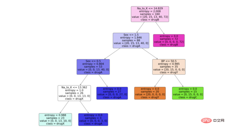
步骤6:可视化模型
现在我们有了决策树模型,让我们利用python中scikit learn包提供的“plot_tree”函数来可视化它。按照代码从python中的决策树模型生成一个漂亮的树图。
Python实现:
feature_names = df.columns[:5] target_names = df['Drug'].unique().tolist() plot_tree(model, feature_names = feature_names, class_names = target_names, filled = True, rounded = True) plt.savefig('tree_visualization.png')输出:
结论
有很多技术和其他算法用于优化决策树和避免过拟合,比如剪枝。虽然决策树通常是不稳定的,这意味着数据的微小变化会导致最优树结构的巨大变化,但其简单性使其成为广泛应用的有力候选。在神经网络流行之前,决策树是机器学习中最先进的算法。其他一些集成模型,比如随机森林模型,比普通决策树模型更强大。
决策树由于其简单性和可解释性而非常强大。决策树和随机森林在用户注册建模、信用评分、故障预测、医疗诊断等领域有着广泛的应用。我为本文提供了完整的代码。
完整代码:
import pandas as pd # 数据处理 import numpy as np # 使用数组 import matplotlib.pyplot as plt # 可视化 from matplotlib import rcParams # 图大小 from termcolor import colored as cl # 文本自定义 from sklearn.tree import DecisionTreeClassifier as dtc # 树算法 from sklearn.model_selection import train_test_split # 拆分数据 from sklearn.metrics import accuracy_score # 模型准确度 from sklearn.tree import plot_tree # 树图 rcParams['figure.figsize'] = (25, 20) df = pd.read_csv('drug.csv') df.drop('Unnamed: 0', axis = 1, inplace = True) print(cl(df.head(), attrs = ['bold'])) df.info() for i in df.Sex.values: if i == 'M': df.Sex.replace(i, 0, inplace = True) else: df.Sex.replace(i, 1, inplace = True) for i in df.BP.values: if i == 'LOW': df.BP.replace(i, 0, inplace = True) elif i == 'NORMAL': df.BP.replace(i, 1, inplace = True) elif i == 'HIGH': df.BP.replace(i, 2, inplace = True) for i in df.Cholesterol.values: if i == 'LOW': df.Cholesterol.replace(i, 0, inplace = True) else: df.Cholesterol.replace(i, 1, inplace = True) print(cl(df, attrs = ['bold'])) X_var = df[['Sex', 'BP', 'Age', 'Cholesterol', 'Na_to_K']].values # 自变量 y_var = df['Drug'].values # 因变量 print(cl('X variable samples : {}'.format(X_var[:5]), attrs = ['bold'])) print(cl('Y variable samples : {}'.format(y_var[:5]), attrs = ['bold'])) X_train, X_test, y_train, y_test = train_test_split(X_var, y_var, test_size = 0.2, random_state = 0) print(cl('X_train shape : {}'.format(X_train.shape), attrs = ['bold'], color = 'red')) print(cl('X_test shape : {}'.format(X_test.shape), attrs = ['bold'], color = 'red')) print(cl('y_train shape : {}'.format(y_train.shape), attrs = ['bold'], color = 'green')) print(cl('y_test shape : {}'.format(y_test.shape), attrs = ['bold'], color = 'green')) model = dtc(criterion = 'entropy', max_depth = 4) model.fit(X_train, y_train) pred_model = model.predict(X_test) print(cl('Accuracy of the model is {:.0%}'.format(accuracy_score(y_test, pred_model)), attrs = ['bold'])) feature_names = df.columns[:5] target_names = df['Drug'].unique().tolist() plot_tree(model, feature_names = feature_names, class_names = target_names, filled = True, rounded = True) plt.savefig('tree_visualization.png')The above is the detailed content of How to build a decision tree in Python. For more information, please follow other related articles on the PHP Chinese website!

Hot AI Tools

Undresser.AI Undress
AI-powered app for creating realistic nude photos

AI Clothes Remover
Online AI tool for removing clothes from photos.

Undress AI Tool
Undress images for free

Clothoff.io
AI clothes remover

AI Hentai Generator
Generate AI Hentai for free.

Hot Article
Hot Tools

Notepad++7.3.1
Easy-to-use and free code editor

SublimeText3 Chinese version
Chinese version, very easy to use

Zend Studio 13.0.1
Powerful PHP integrated development environment

Dreamweaver CS6
Visual web development tools

SublimeText3 Mac version
God-level code editing software (SublimeText3)
Hot Topics
 1378
1378
 52
52

 PHP and Python: Code Examples and Comparison
Apr 15, 2025 am 12:07 AM
PHP and Python: Code Examples and Comparison
Apr 15, 2025 am 12:07 AM
PHP and Python have their own advantages and disadvantages, and the choice depends on project needs and personal preferences. 1.PHP is suitable for rapid development and maintenance of large-scale web applications. 2. Python dominates the field of data science and machine learning.
 How to train PyTorch model on CentOS
Apr 14, 2025 pm 03:03 PM
How to train PyTorch model on CentOS
Apr 14, 2025 pm 03:03 PM
Efficient training of PyTorch models on CentOS systems requires steps, and this article will provide detailed guides. 1. Environment preparation: Python and dependency installation: CentOS system usually preinstalls Python, but the version may be older. It is recommended to use yum or dnf to install Python 3 and upgrade pip: sudoyumupdatepython3 (or sudodnfupdatepython3), pip3install--upgradepip. CUDA and cuDNN (GPU acceleration): If you use NVIDIAGPU, you need to install CUDATool
 Detailed explanation of docker principle
Apr 14, 2025 pm 11:57 PM
Detailed explanation of docker principle
Apr 14, 2025 pm 11:57 PM
Docker uses Linux kernel features to provide an efficient and isolated application running environment. Its working principle is as follows: 1. The mirror is used as a read-only template, which contains everything you need to run the application; 2. The Union File System (UnionFS) stacks multiple file systems, only storing the differences, saving space and speeding up; 3. The daemon manages the mirrors and containers, and the client uses them for interaction; 4. Namespaces and cgroups implement container isolation and resource limitations; 5. Multiple network modes support container interconnection. Only by understanding these core concepts can you better utilize Docker.
 How is the GPU support for PyTorch on CentOS
Apr 14, 2025 pm 06:48 PM
How is the GPU support for PyTorch on CentOS
Apr 14, 2025 pm 06:48 PM
Enable PyTorch GPU acceleration on CentOS system requires the installation of CUDA, cuDNN and GPU versions of PyTorch. The following steps will guide you through the process: CUDA and cuDNN installation determine CUDA version compatibility: Use the nvidia-smi command to view the CUDA version supported by your NVIDIA graphics card. For example, your MX450 graphics card may support CUDA11.1 or higher. Download and install CUDAToolkit: Visit the official website of NVIDIACUDAToolkit and download and install the corresponding version according to the highest CUDA version supported by your graphics card. Install cuDNN library:
 Python vs. JavaScript: Community, Libraries, and Resources
Apr 15, 2025 am 12:16 AM
Python vs. JavaScript: Community, Libraries, and Resources
Apr 15, 2025 am 12:16 AM
Python and JavaScript have their own advantages and disadvantages in terms of community, libraries and resources. 1) The Python community is friendly and suitable for beginners, but the front-end development resources are not as rich as JavaScript. 2) Python is powerful in data science and machine learning libraries, while JavaScript is better in front-end development libraries and frameworks. 3) Both have rich learning resources, but Python is suitable for starting with official documents, while JavaScript is better with MDNWebDocs. The choice should be based on project needs and personal interests.
 How to choose the PyTorch version under CentOS
Apr 14, 2025 pm 02:51 PM
How to choose the PyTorch version under CentOS
Apr 14, 2025 pm 02:51 PM
When selecting a PyTorch version under CentOS, the following key factors need to be considered: 1. CUDA version compatibility GPU support: If you have NVIDIA GPU and want to utilize GPU acceleration, you need to choose PyTorch that supports the corresponding CUDA version. You can view the CUDA version supported by running the nvidia-smi command. CPU version: If you don't have a GPU or don't want to use a GPU, you can choose a CPU version of PyTorch. 2. Python version PyTorch
 How to install nginx in centos
Apr 14, 2025 pm 08:06 PM
How to install nginx in centos
Apr 14, 2025 pm 08:06 PM
CentOS Installing Nginx requires following the following steps: Installing dependencies such as development tools, pcre-devel, and openssl-devel. Download the Nginx source code package, unzip it and compile and install it, and specify the installation path as /usr/local/nginx. Create Nginx users and user groups and set permissions. Modify the configuration file nginx.conf, and configure the listening port and domain name/IP address. Start the Nginx service. Common errors need to be paid attention to, such as dependency issues, port conflicts, and configuration file errors. Performance optimization needs to be adjusted according to the specific situation, such as turning on cache and adjusting the number of worker processes.
 How to do data preprocessing with PyTorch on CentOS
Apr 14, 2025 pm 02:15 PM
How to do data preprocessing with PyTorch on CentOS
Apr 14, 2025 pm 02:15 PM
Efficiently process PyTorch data on CentOS system, the following steps are required: Dependency installation: First update the system and install Python3 and pip: sudoyumupdate-ysudoyuminstallpython3-ysudoyuminstallpython3-pip-y Then, download and install CUDAToolkit and cuDNN from the NVIDIA official website according to your CentOS version and GPU model. Virtual environment configuration (recommended): Use conda to create and activate a new virtual environment, for example: condacreate-n
