

How to sum columns in Excel

How to quickly view the sum of a column in Excel
If you just want to know the sum of a column without adding that information to the spreadsheet, you can use the Excel status bar to quickly view a column or any cell The sum of the grid areas.
To see the sum of a column using the Excel status bar:
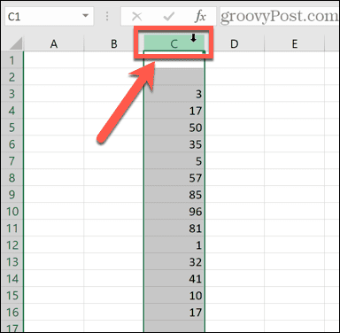
- Highlight the data you want to summarize. To select an entire column, click the column name. Otherwise, drag cells to select your range.

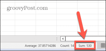
- At the bottom of the screen, you'll see information about your selection, such as the average of all values and the number of data points in the range. You will also see the sum of all values in the selected cells.
How to use AutoSum to sum columns in Excel
If you wish to add the sum of a column to a spreadsheet, in many cases , you can do this fastest by using the AutoSum function. This will automatically select a range of values for you.
However, in some cases, such as a mix of numeric and text entries, the range it selects may not be quite right and you will need to fix it manually.
Use AutoSum to sum columns:
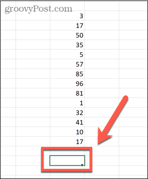
- Click the cell where you want the sum to appear. This should be in the same column as the data you are asking to sum.
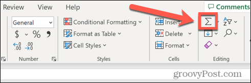
- In the Homepage toolbar, click the AutoSum button.
- You can also use the keyboard shortcut Alt = (hold Alt and press equal sign).
- You can also use the keyboard shortcut Alt = (hold Alt and press equal sign).
- The cells you select will be populated with a formula that includes the SUM function and a range from the same column. Cells within the range will also be highlighted.
- When you are satisfied with the range of cells selected by AutoSum, press Enter to apply the formula. If the range isn't what you want, you can drag out a different range and press Enter.
- The sum of the values in the column will now be displayed.
How to use the SUM function to sum columns in Excel
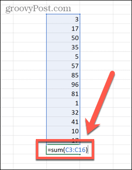
If your data contains both values and text, the AutoSum function will select that column The value below the last text value in .
You can manually create a formula using the SUM function to select your own range and ensure that you sum all values in the column.
Use the SUM function to sum columns:
- Click the cell where you want the sum to appear. This can be any cell you choose - it doesn't have to be in the same column.
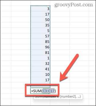
- Enter =SUM(
- Drag out the range of cells you want to include or click a column name to select the entire column.
- Type Close the bracket at the end and press Enter.
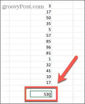
- Your sum will now be calculated. If any of the selected cells contain text, these will be ignored. However , all values will be included.
How to sum columns in Excel using named ranges
If you are working with large amounts of data, highlight Large numbers of cells can be time-consuming. However, it is possible to apply names to specific ranges of data. You can simply reference the range in your formulas by naming it without having to select all the data each time.
Sum columns using named ranges:
- Highlight the data range to be named.
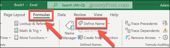
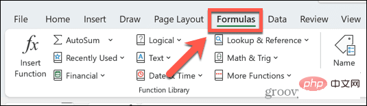
- Under the Formula menu, click Define Name.
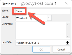
- Enter a name for your range and click OK.
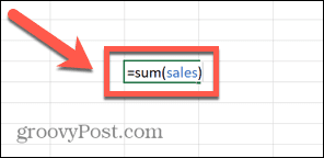
- Select the cell where you want the sum to appear and type =SUM( followed by the range name and the closing parenthesis. For example, =SUM(sales).
- Press Enter key and Excel will calculate the sum of your named range.
How to use SUBTOTAL to sum a filtered column
The SUM function is not of much use if you are working with filtered data. Even if you use a data filter to display only certain values, the SUM function calculates the sum of all visible and hidden values.
If you only want to find the sum of those values returned by the filter, you need to use the SUBTOTAL function.
To use the SUBTOTAL function to filter a column in Excel Sum:
- Highlight your cells.
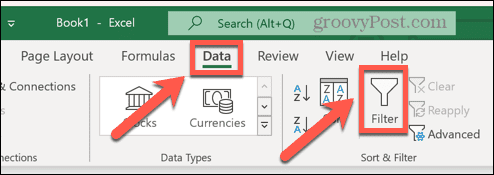
- In the Data menu, click the Filter icon .
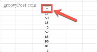
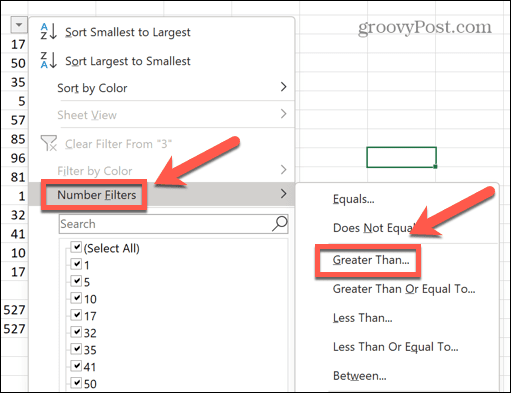
- Click the filter arrow at the top of the data column.
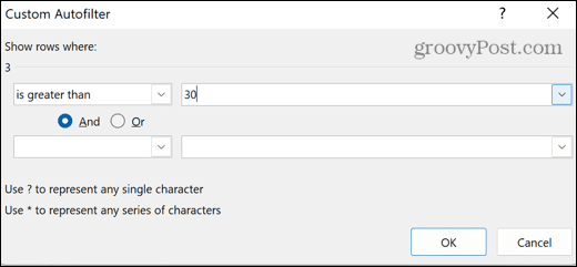
- Set the filter of your choice.
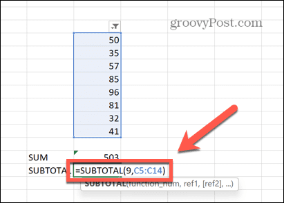
- Select the cells where you want the subtotal to appear.
- Type =SUBTOTAL(9,Then select the visible Cell . 9 is part of the function and means you are looking for the sum of the values
- Type the final closing bracket.
- Press Enter.
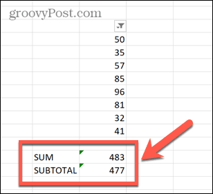
- Subtotal will show the correct sum of the visible values in the filtered data. In contrast, using the SUM function gives you the sum of all visible cells, plus the top and bottom of your selection Any hidden cells between cells.
How to sum columns using an Excel table
Although the data in the spreadsheet is in tabular form stored, but you can convert the data into an Excel table. You can quickly change the styles in the Excel table, and you can also reference them directly in formulas.
You can also use the table design tool to quickly summarize a column of data .
To sum columns using an Excel table:
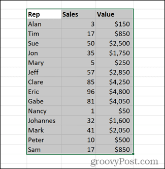
- Highlight the data you want to convert to an Excel table.
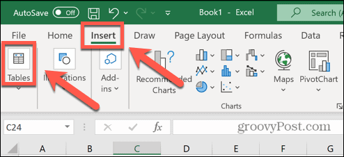
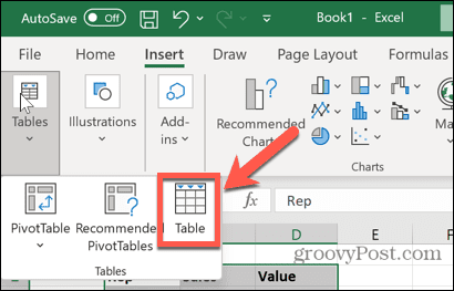
- Under the Insert menu, click Table.
- Select Table.
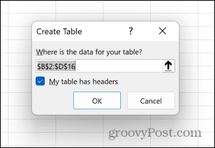
- Make sure the range is correct and if you include headers in the selection, make sure My table has headers is checked.
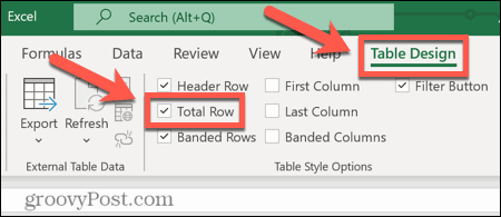
- After creating the Excel table, Please make sure the Total Row option is selected in the Table Design menu.
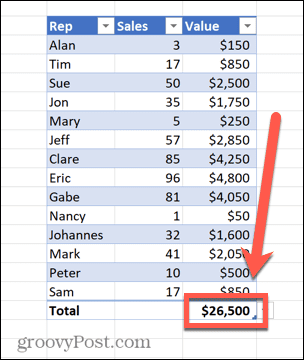
- will add a new row to the table, displaying the table The sum of the values in the last column.
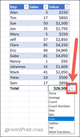
- If you wish, you can click the down arrow next to the value to change it from a sum to a variety of other calculations.
Become an Excel Pro
Even something as simple as summing columns in Excel has multiple ways to do it, as the above steps illustrate. Show. Although many people have only scratched the surface of Excel's capabilities, it is still a very powerful application.
The above is the detailed content of How to sum columns in Excel. For more information, please follow other related articles on the PHP Chinese website!

Hot AI Tools

Undresser.AI Undress
AI-powered app for creating realistic nude photos

AI Clothes Remover
Online AI tool for removing clothes from photos.

Undress AI Tool
Undress images for free

Clothoff.io
AI clothes remover

AI Hentai Generator
Generate AI Hentai for free.

Hot Article
Hot Tools

Notepad++7.3.1
Easy-to-use and free code editor

SublimeText3 Chinese version
Chinese version, very easy to use

Zend Studio 13.0.1
Powerful PHP integrated development environment

Dreamweaver CS6
Visual web development tools

SublimeText3 Mac version
God-level code editing software (SublimeText3)
Hot Topics
 1377
1377
 52
52

 How to fix formula parsing errors in Google Sheets
May 05, 2023 am 11:52 AM
How to fix formula parsing errors in Google Sheets
May 05, 2023 am 11:52 AM
What are formula parsing errors in Google Sheets? Formula parsing errors occur in Google Sheets when the application cannot handle the instructions in the formula. This is usually because there's a problem with the formula itself, or there's a problem with the cells the formula refers to. There are many different types of formula parsing errors in Google Sheets. The method for fixing formula parsing errors in Google Sheets depends on the type of error your formula produces. We'll look at some of the most common formula parsing errors below and how to fix them. How to fix #ERROR! Error in Google Sheets #Error! Formula parsing errors occur when Google Sheets doesn't understand your formula but isn't sure what the problem is. When you are on the spreadsheet
 Excel found a problem with one or more formula references: How to fix it
Apr 17, 2023 pm 06:58 PM
Excel found a problem with one or more formula references: How to fix it
Apr 17, 2023 pm 06:58 PM
Use an Error Checking Tool One of the quickest ways to find errors with your Excel spreadsheet is to use an error checking tool. If the tool finds any errors, you can correct them and try saving the file again. However, the tool may not find all types of errors. If the error checking tool doesn't find any errors or fixing them doesn't solve the problem, then you need to try one of the other fixes below. To use the error checking tool in Excel: select the Formulas tab. Click the Error Checking tool. When an error is found, information about the cause of the error will appear in the tool. If it's not needed, fix the error or delete the formula causing the problem. In the Error Checking Tool, click Next to view the next error and repeat the process. When not
 How to set the print area in Google Sheets?
May 08, 2023 pm 01:28 PM
How to set the print area in Google Sheets?
May 08, 2023 pm 01:28 PM
How to Set GoogleSheets Print Area in Print Preview Google Sheets allows you to print spreadsheets with three different print areas. You can choose to print the entire spreadsheet, including each individual worksheet you create. Alternatively, you can choose to print a single worksheet. Finally, you can only print a portion of the cells you select. This is the smallest print area you can create since you could theoretically select individual cells for printing. The easiest way to set it up is to use the built-in Google Sheets print preview menu. You can view this content using Google Sheets in a web browser on your PC, Mac, or Chromebook. To set up Google
 How to solve out of memory problem in Microsoft Excel?
Apr 22, 2023 am 10:04 AM
How to solve out of memory problem in Microsoft Excel?
Apr 22, 2023 am 10:04 AM
Microsoft Excel is a popular program used for creating worksheets, data entry operations, creating graphs and charts, etc. It helps users organize their data and perform analysis on this data. As can be seen, all versions of the Excel application have memory issues. Many users have reported seeing the error message "Insufficient memory to run Microsoft Excel. Please close other applications and try again." when trying to open Excel on their Windows PC. Once this error is displayed, users will not be able to use MSExcel as the spreadsheet will not open. Some users reported problems opening Excel downloaded from any email client
 5 Tips to Fix Stdole32.tlb Excel Error in Windows 11
May 09, 2023 pm 01:37 PM
5 Tips to Fix Stdole32.tlb Excel Error in Windows 11
May 09, 2023 pm 01:37 PM
When you start Microsoft Word or Microsoft Excel, Windows very tediously tries to set up Office 365. At the end of the process, you may receive a Stdole32.tlbExcel error. Since there are many bugs in the Microsoft Office suite, launching any of its products can sometimes be a nightmare. Microsoft Office is a software that is used regularly. Microsoft Office has been available to consumers since 1990. Starting from Office 1.0 version and developing to Office 365, this
 How to display the Developer tab in Microsoft Excel
Apr 14, 2023 pm 02:10 PM
How to display the Developer tab in Microsoft Excel
Apr 14, 2023 pm 02:10 PM
If you need to record or run macros, insert Visual Basic forms or ActiveX controls, or import/export XML files in MS Excel, you need the Developer tab in Excel for easy access. However, this developer tab does not appear by default, but you can add it to the ribbon by enabling it in Excel options. If you are working with macros and VBA and want to easily access them from the Ribbon, continue reading this article. Steps to enable Developer tab in Excel 1. Launch MS Excel application. Right-click anywhere on one of the top ribbon tabs and when
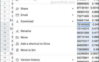
 How to embed a PDF document in an Excel worksheet
May 28, 2023 am 09:17 AM
How to embed a PDF document in an Excel worksheet
May 28, 2023 am 09:17 AM
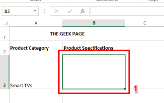
It is usually necessary to insert PDF documents into Excel worksheets. Just like a company's project list, we can instantly append text and character data to Excel cells. But what if you want to attach the solution design for a specific project to its corresponding data row? Well, people often stop and think. Sometimes thinking doesn't work either because the solution isn't simple. Dig deeper into this article to learn how to easily insert multiple PDF documents into an Excel worksheet, along with very specific rows of data. Example Scenario In the example shown in this article, we have a column called ProductCategory that lists a project name in each cell. Another column ProductSpeci
 How to remove commas from numeric and text values in Excel
Apr 17, 2023 pm 09:01 PM
How to remove commas from numeric and text values in Excel
Apr 17, 2023 pm 09:01 PM
On numeric values, on text strings, using commas in the wrong places can really get annoying, even for the biggest Excel geeks. You may even know how to get rid of commas, but the method you know may be time-consuming for you. Well, no matter what your problem is, if it is related to a comma in the wrong place in your Excel worksheet, we can tell you one thing, all your problems will be solved today, right here! Dig deeper into this article to learn how to easily remove commas from numbers and text values in the simplest steps possible. Hope you enjoy reading. Oh, and don’t forget to tell us which method catches your eye the most! Section 1: How to Remove Commas from Numerical Values When a numerical value contains a comma, there are two possible situations: