Comparative analysis of deep learning architectures
The concept of deep learning originates from the research of artificial neural networks. A multi-layer perceptron containing multiple hidden layers is a deep learning structure. Deep learning combines low-level features to form more abstract high-level representations to represent categories or characteristics of data. It is able to discover distributed feature representations of data. Deep learning is a type of machine learning, and machine learning is the only way to achieve artificial intelligence.
So, what are the differences between various deep learning system architectures?
1. Fully Connected Network (FCN)
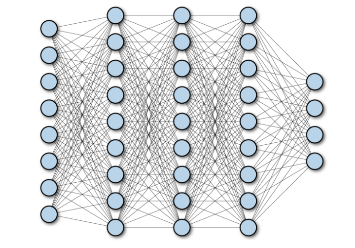
Fully Connected Network (FCN) consists of a series of fully connected layers, with each neuron in each layer connected to another layer each neuron in . Its main advantage is that it is "structure agnostic", i.e. no special assumptions about the input are required. While this structure agnostic makes fully connected networks very broadly applicable, such networks tend to perform weaker than specialized networks tuned specifically to the structure of the problem space.
The following figure shows a multi-layer depth fully connected network:
2. Convolutional Neural Network (CNN)
Convolutional Neural Network (CNN) is a multi-layer neural network architecture mainly used in image processing applications. The CNN architecture explicitly assumes that the input has spatial dimensions (and optionally depth dimensions), such as images, which allows certain properties to be encoded into the model architecture. Yann LeCun created the first CNN, an architecture originally used to recognize handwritten characters.
2.1 Architectural features of CNN
Break down the technical details of the computer vision model using CNN:
- Input of the model: The input of the CNN model is usually an image or text. CNNs can also be used on text, but they are usually less used.
The image is represented here as a grid of pixels, which is a grid of positive integers, with each number assigned a color.
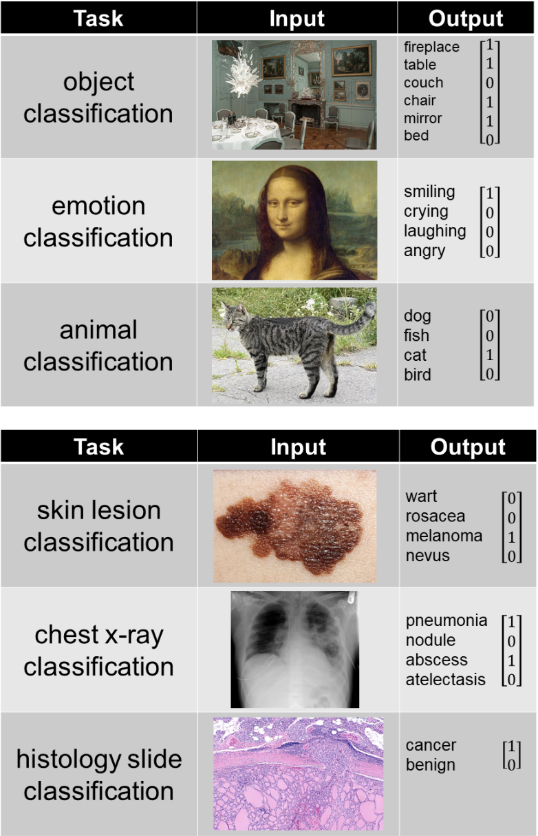
- Output of the model: The output of the model depends on what it is trying to predict, the following examples represent some common tasks:
-

A simple convolutional neural network consists of a series of layers, each layer transforms an activation volume into another representation through a differentiable function. The architecture of a convolutional neural network mainly uses three types of layers: convolutional layers, pooling layers, and fully connected layers. The image below shows the different parts of a convolutional neural network layer:
- Convolution: A convolution filter scans the image, using addition and multiplication operations. CNN attempts to learn the values in the convolutional filters to predict the desired output.
- Nonlinearity: This is the equation applied to the convolutional filter, which allows the CNN to learn complex relationships between input and output images.
- Pooling: Also known as "max pooling", it only selects the largest number in a series of numbers. This helps reduce the size of the expression and reduces the amount of calculations the CNN must perform, improving efficiency.
The combination of these three operations forms a fully convolutional network.
2.2 Use cases of CNN
CNN (Convolutional Neural Network) is a neural network commonly used to solve problems related to spatial data, usually for images (2D CNN) and audio ( 1D CNN) and other fields. The wide range of applications of CNN include face recognition, medical analysis and classification, etc. Through CNN, more detailed features can be captured in image or audio data, thereby achieving more accurate recognition and analysis. In addition, CNN can also be applied to other fields, such as natural language processing and time series data. In short, CNN can help us better understand and analyze various types of data.
2.3 Advantages of CNN over FCN
Parameter sharing/computation feasibility:
Since CNN uses parameter sharing, the number of weights in CNN and FCN architectures usually differs by several orders of magnitude .
For a fully connected neural network, there is an input with a shape of (Hin×Win×Cin) and an output with a shape of (Hout×Wout×Cout). This means that every pixel color of the output feature is connected to every pixel color of the input feature. For each pixel of the input and output images, there is an independent learnable parameter. Therefore, the number of parameters is (Hin×Hout×Win×Wout×Cin×Cout).
In the convolutional layer, the input is an image of shape (Hin, Win, Cin), and the weights consider the neighborhood size of the given pixel to be K×K. The output is the weighted sum of a given pixel and its neighbors. There is a separate kernel for each pair (Cin, Cout) of input and output channels, but the weights of the kernel are position-independent tensors of shape (K, K, Cin, Cout). In fact, this layer can accept images of any resolution, while fully connected layers can only use fixed resolutions. Finally, the layer parameters are (K, K, Cin, Cout). For the case where the kernel size K is much smaller than the input resolution, the number of variables will be significantly reduced.
Since AlexNet won the ImageNet competition, the fact that every winning neural network has used a CNN component proves that CNNs are more effective for image data. It is very likely that you will not find any meaningful comparison because it is not feasible to use only FC layers to process image data, while CNN can process this data. why?
The number of weights with 1000 neurons in the FC layer is approximately 150 million for the image. This is just the number of weights for a layer. Modern CNN architectures have 50-100 layers with a total of hundreds of thousands of parameters (for example, ResNet50 has 23M parameters, Inception V3 has 21M parameters).
From a mathematical point of view, comparing the number of weights between CNN and FCN (with 100 hidden units), if the input image is 500×500×3:
- FC layer Wx = 100×(500×500×3)=100×750000=75M
- CNN layer =
<code>((shape of width of the filter * shape of height of the filter * number of filters in the previous layer+1)*number of filters)( +1 是为了偏置) = (Fw×Fh×D+1)×F=(5×5×3+1)∗2=152</code>
Translation invariance
Invariance refers to An object can still be correctly identified even if its position changes. This is usually a positive feature because it maintains the identity (or category) of the object. "Translation" here has a specific meaning in geometry. The image below shows the same object in different locations, and due to translation invariance, the CNN is able to correctly identify that they are both cats.
3. Recurrent Neural Network (RNN)
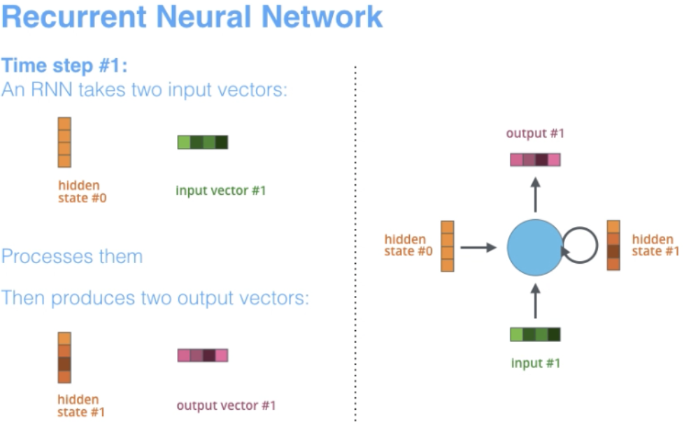
RNN is one of the basic network architectures on which other deep learning architectures are built. A key difference is that unlike normal feedforward networks, RNNs can have connections that feed back to their previous or same layer. In a sense, RNN has a "memory" of previous computations and uses this information for current processing.
3.1 Architectural Features of RNN
The term "Recurrent" applies to the network performing the same task on each sequence instance , so the output depends on previous calculations and results.
RNN is naturally suitable for many NLP tasks, such as language modeling. They are able to capture the difference in meaning between "dog" and "hot dog", so RNNs are tailor-made for modeling this kind of context dependence in languages and similar sequence modeling tasks, which makes using RNNs in these areas rather than The main reason for CNN. Another advantage of RNN is that the model size does not increase with the input size, so it is possible to handle inputs of arbitrary length.
In addition, unlike CNN, RNN has flexible calculation steps, provides better modeling capabilities, and creates the possibility of capturing unlimited context because it takes into account historical information and its weights are in Time is shared. However, recurrent neural networks suffer from the vanishing gradient problem. The gradient becomes very small, thus making the update weights of backpropagation very small. Due to the sequential processing required for each label and the presence of vanishing/exploding gradients, RNN training is slow and sometimes difficult to converge.
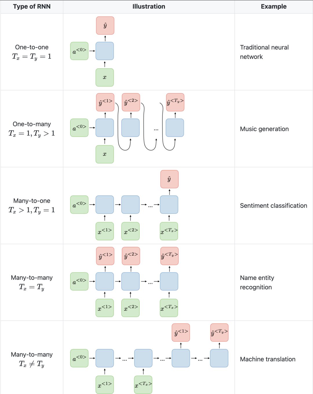
The picture below from Stanford University is an example of RNN architecture.
Another thing to note is that CNN and RNN have different architectures. CNN is a feed-forward neural network that uses filters and pooling layers, while RNN feeds the results back into the network through autoregression.
3.2 Typical use cases of RNN
RNN is a neural network specifically designed to analyze time series data. Among them, time series data refers to data arranged in time order, such as text or video. RNN has wide applications in text translation, natural language processing, sentiment analysis, and speech analysis. For example, it can be used to analyze audio recordings in order to identify the speaker's speech and convert it into text. Additionally, RNNs can also be used for text generation, such as creating text for emails or social media posts.
3.3 Comparative advantages of RNN and CNN
In CNN, the input and output sizes are fixed. This means that the CNN takes a fixed size image and outputs it to the appropriate level, along with the confidence of its prediction. However, in RNN, the input and output sizes may vary. This feature is useful for applications that require variable-sized input and output, such as generating text.
Both Gated Recurrent Units (GRU) and Long Short-Term Memory Units (LSTM) provide solutions to the vanishing gradient problem encountered by Recurrent Neural Networks (RNN).
4. Long short memory neural network (LSTM)
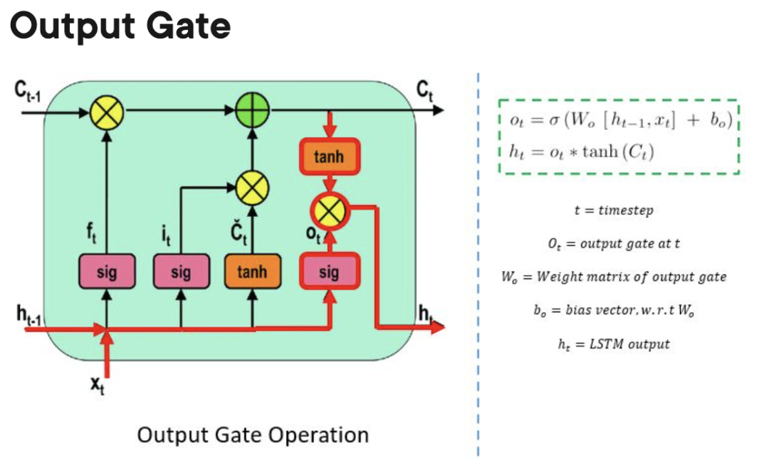
Long short memory neural network (LSTM) is a special type of RNN. It makes it easier for RNNs to retain information over many timestamps by learning long-term dependencies. The figure below is a visual representation of the LSTM architecture.
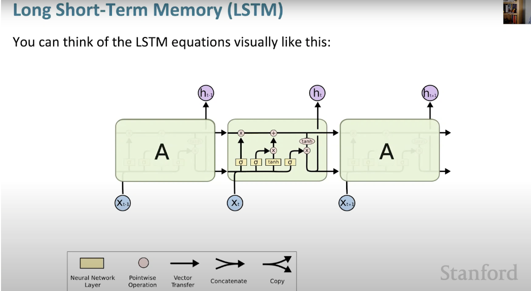
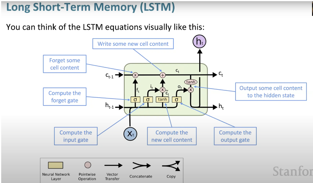
LSTM is ubiquitous and can be found in many applications or products , such as a smartphone. Its power lies in the fact that it moves away from the typical neuron-based architecture and instead adopts the concept of memory units. This memory unit retains its value according to the function of its input, and can hold its value for a short or long time. This allows the unit to remember important things, not just the last calculated value.
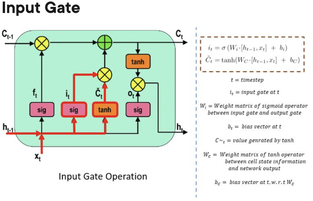
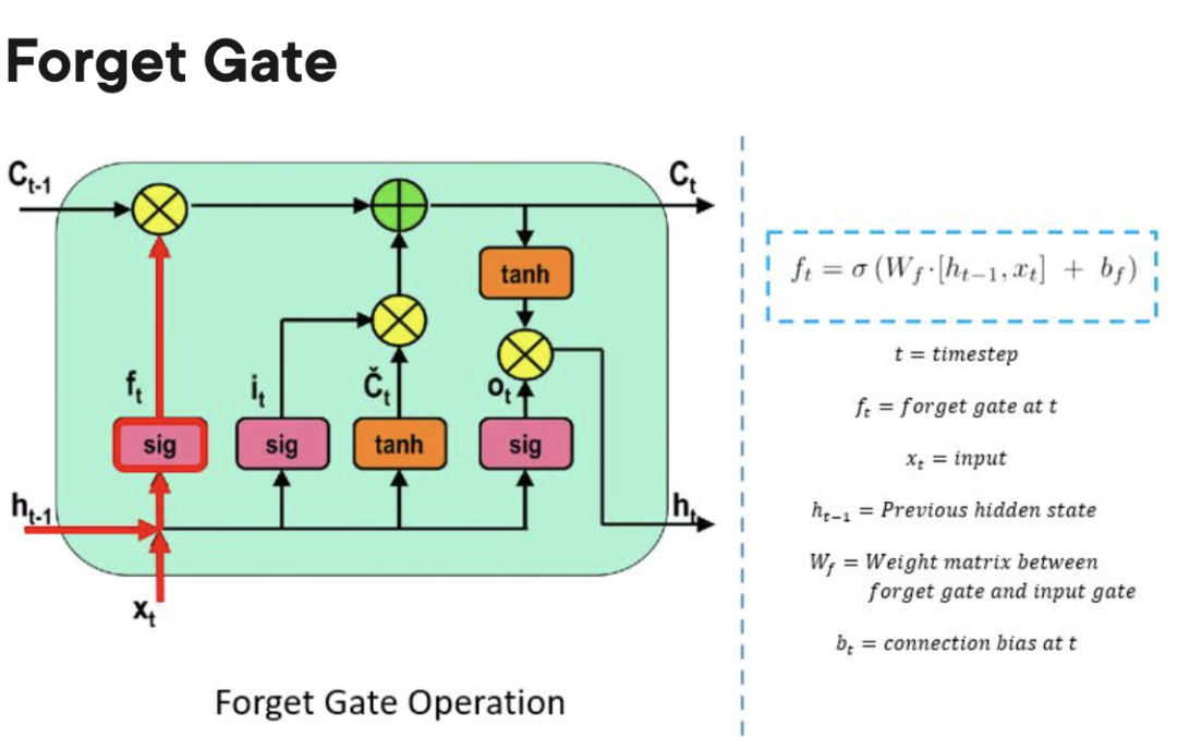
The LSTM memory unit contains three gates that control the inflow or outflow of information within its unit.
- Input Gate: Controls when information can flow into memory.
Forgetting Gate: Responsible for tracking which information can be "forgotten" to make room for the processing unit to remember new data.
Output Gate: Determines when information stored within a processing unit can be used as the output of the cell.
The advantages and disadvantages of LSTM compared to GRU and RNN
Compared to GRU and Especially RNN, LSTM can learn longer-term dependencies. Since there are three gates (two in GRU and zero in RNN), LSTM has more parameters compared to RNN and GRU. These additional parameters allow the LSTM model to better handle complex sequence data, such as natural language or time series data. Furthermore, LSTMs can also handle variable-length input sequences because their gate structure allows them to ignore unnecessary inputs. As a result, LSTM performs well in many applications, including speech recognition, machine translation, and stock market predictions.
5. Gated Recurrent Unit (GRU)
GRU has two gates: update gate and reset gate (essentially two vectors) to decide what information should be passed to the output .
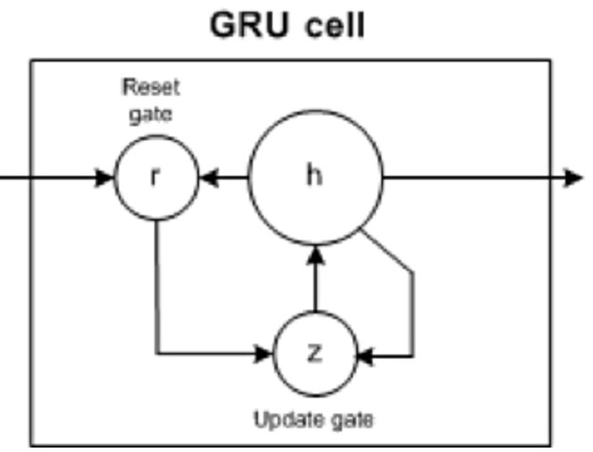
- Reset gate: Helps the model decide how much past information it can forget.
- Update gate: Helps the model determine how much past information (previous time steps) needs to be passed to the future.
The advantages and disadvantages of GRU comparing LSTM and RNN
Similar to RNN, GRU is also a recurrent neural network, which can effectively retain information for a long time and capture longer than RNN Dependencies. However, GRU is simpler and faster to train than LSTM.
Although GRU is more complex in implementation than RNN, since it only contains two gating mechanisms, it has a smaller number of parameters and generally cannot capture longer range dependencies like LSTM. Therefore, GRU may require more training data in some cases to achieve the same performance level as LSTM.
In addition, because GRU is relatively simple and its computational cost is low, it may be more appropriate to use GRU in resource-limited environments, such as mobile devices or embedded systems. On the other hand, if the accuracy of the model is critical to the application, LSTM may be a better choice.
6.Transformer
The paper on Transformers "Attention is All You Need" is almost the number one paper ever on Arxiv. Transformer is a large encoder-decoder model capable of processing entire sequences using complex attention mechanisms.
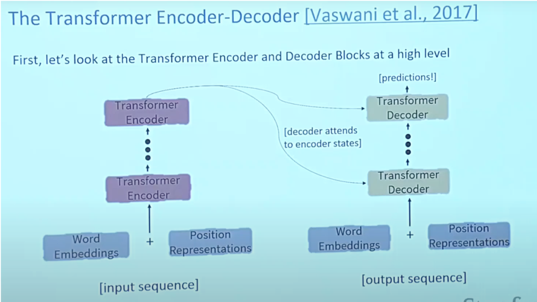
# Typically, in natural language processing applications, each input word is first converted into a vector using an embedding algorithm. Embedding only happens in the lowest level encoder. The abstraction shared by all encoders is that they receive a list of vectors of size 512, which will be the word embeddings, but in other encoders it will be directly below the encoder output.
Attention provides a solution to the bottleneck problem. For these types of models, context vectors become a bottleneck, making it difficult for the model to handle long sentences. Attention allows the model to focus on relevant parts of the input sequence as needed and treat the representation of each word as a query to access and combine information from a set of values.
6.1 Transformer architectural features
Generally, in the Transformer architecture, the encoder can pass all hidden states to the decoder. However, the decoder uses attention to perform an additional step before generating the output. The decoder multiplies each hidden state by its softmax score, thereby amplifying higher-scoring hidden states and flooding other hidden states. This allows the model to focus on the parts of the input that are relevant to the output.
Self-attention is located in the encoder. The first step is to create 3 vectors from each encoder input vector (embedding of each word): Key, Query and Value vectors. These vectors are obtained by converting the embedding Created by multiplying the 3 matrices trained during training. The K, V, Q dimensions are 64, while the embedding and encoder input/output vectors have a dimension of 512. The picture below is from Jay Alammar's Illustrated Transformer, which is probably the best visual interpretation on the Internet.

The size of this list is a hyperparameter that can be set and will basically be the length of the longest sentence in the training data set.
- Attention:
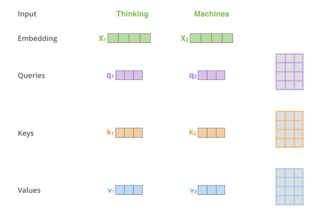
What are query, key and value vectors? They are abstract concepts useful when calculating and thinking about attention. The calculation of cross-attention in the decoder is the same as that of self-attention except for the input. Cross-attention asymmetrically combines two independent embedding sequences of the same dimension, while the input of self-attention is a single embedding sequence.
In order to discuss Transformer, it is also necessary to discuss two pre-trained models, namely BERT and GPT, because they led to the success of Transformer.
GPT's pre-trained decoder has 12 layers, including 768-dimensional hidden states, 3072-dimensional feed-forward hidden layers, and is encoded with 40,000 merged byte pairs. It is mainly used in natural language reasoning to mark sentence pairs as entailment, contradiction, or neutral.
BERT is a pre-trained encoder that uses masked language modeling to replace a portion of the words in the input with special [MASK] tokens and then try to predict those words. Therefore, the loss only needs to be calculated on the predicted masked words. Both BERT model sizes have a large number of encoder layers (called Transformer blocks in the paper) - 12 in the Base version and 24 in the Large version. These also have larger feedforward networks (768 and 1024 hidden units respectively) and more than the default configuration in the Transformer reference implementation in the initial paper (6 encoder layers, 512 hidden units and 8 attention heads) of attention heads (12 and 16 respectively). BERT models are easy to fine-tune and can usually be done on a single GPU. BERT can be used for translation in NLP, especially low-resource language translation.
One performance drawback of Transformers is that their computation time in self-attention is quadratic, while RNNs only grow linearly.
6.2 Transformer use cases
6.2.1 Language field
In traditional language models, adjacent words are first grouped together, while Transformer can be parallelized Processing so that every element in the input data is connected to or attended to every other element. This is called "self-attention." This means that the Transformer can see the contents of the entire data set as soon as it starts training.
Before the emergence of Transformer, the progress of AI language tasks lagged behind the development of other fields to a large extent. In fact, in the deep learning revolution of the past 10 years or so, natural language processing was a latecomer, and NLP lagged behind computer vision to some extent. However, with the emergence of Transformers, the NLP field has received a huge boost and a series of models have been launched that achieve good results in various NLP tasks.
For example, in order to understand the difference between traditional language models (based on recursive architectures such as RNN, LSTM or GRU) and Transformers, we can give an example: "The owl spied a squirrel. It tried to grab it with its talons but only got the end of its tail." The structure of the second sentence is confusing: what does that "it" mean? Traditional language models that only focus on the words surrounding "it" would have difficulty, but a Transformer that connects each word to every other word can tell that an owl caught a squirrel, and that the squirrel lost part of its tail.
6.2.2 Vision field
In CNN, we start from the local and gradually obtain the global perspective. CNN recognizes images pixel by pixel by building features from local to global to identify features such as corners or lines. However, in the transformer, through self-attention, connections between remote image locations are established even at the first level of information processing (just like language). If the CNN approach is like scaling starting from a single pixel, then the transformer will gradually bring the entire blurred image into focus.
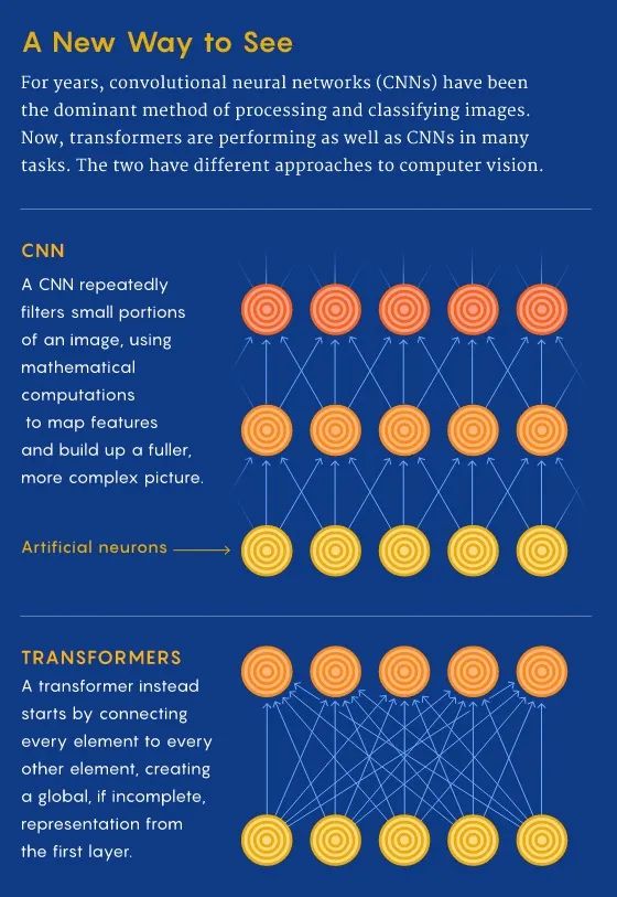
CNN generates local feature representations by repeatedly applying filters on local patches of the input data, gradually increasing their receptive field of view and constructing the global Feature representation. It’s because of convolution that the Photos app can distinguish pears from clouds. Before the transformer architecture, CNN was considered indispensable for vision tasks.
The architecture of the Vision Transformer model is almost identical to the first transformer proposed in 2017, with only some minor changes that enable it to analyze images instead of words. Since language tends to be discrete, the input image needs to be discretized to enable the transformer to process visual input. Exactly imitating the language approach and performing self-attention on every pixel would become prohibitively expensive in computational time. Therefore, ViT divides larger images into square cells or patches (similar to tokens in NLP). The size is arbitrary because the token can be larger or smaller depending on the resolution of the original image (default is 16x16 pixels). But by processing pixels in groups and applying self-attention to each pixel, ViT can quickly process huge training data sets and output increasingly accurate classifications.
6.2.3 Multi-modal tasks
Compared with Transformer, other deep learning architectures only have one skill, while multi-modal learning requires processing different modes in a smooth architecture modal and has a very high relational induction bias to reach the level of human intelligence. In other words, there was a need for a single multipurpose architecture that could seamlessly transition between senses such as reading/viewing, speaking, and listening.
For multi-modal tasks, multiple types of data need to be processed simultaneously, such as original images, videos, and languages, and Transformer provides the potential of a general architecture.

This was a difficult task to accomplish due to the discrete approach taken in earlier architectures, where each type of data had its own specific model Task. However, Transformers provide an easy way to combine multiple input sources. For example, multimodal networks could power systems that read people's lip movements and listen to their voices using rich representations of language and image information simultaneously. Through cross-attention, Transformer is able to derive query, key and value vectors from different sources, making it a powerful tool for multi-modal learning.
Therefore, Transformer is a big step towards the "fusion" of neural network architectures, which can help achieve universal processing of multiple modal data.
6.3 Advantages and disadvantages of Transformer compared to RNN/GRU/LSTM
Compared with RNN/GRU/LSTM, Transformer can learn longer than RNN and its variants (such as GRU and LSTM) Dependencies.
However, the biggest benefit comes from how Transformer is suitable for parallelization. Unlike an RNN that processes one word at each time step, a key property of the Transformer is that the word at each position flows through the encoder via its own path. In the self-attention layer, there are dependencies between these paths as the self-attention layer calculates the importance of other words in each input sequence to that word. However, once the self-attention output is generated, the feedforward layer does not have these dependencies, so individual paths can execute in parallel as they pass through the feedforward layer. This is a particularly useful feature in the case of the Transformer encoder, which processes each input word in parallel with other words after a self-attention layer. However, this feature is not very important for the decoder, since it only generates one word at a time and does not use parallel word paths.
The running time of the Transformer architecture scales quadratically with the length of the input sequence, which means that processing can be slow when processing long documents or characters as input. In other words, during self-attention formation, all interaction pairs need to be calculated, which means that the calculation grows quadratically with the sequence length, that is, O(T^2 d), where T is the sequence length and D is the dimension. For example, corresponding to a simple sentence d=1000, T≤30⇒T^2≤900⇒T^2d≈900K. And for the circulating nerves, it only grows in a linear fashion.
Wouldn’t it be nice if the Transformer didn’t need to compute pairwise interactions between every pair of words in the sentence? There are studies showing that quite high performance levels can be achieved without computing interactions between all word pairs (e.g. by approximating pairwise attention).
Compared with CNN, Transformer has extremely high data requirements. CNNs are still sample efficient, which makes them an excellent choice for low-resource tasks. This is especially true for image/video generation tasks, which even for CNN architectures require large amounts of data (thus implying the extremely high data requirements of the Transformer architecture). For example, the CLIP architecture recently proposed by Radford et al. is trained using CNN-based ResNets as the visual backbone (instead of the ViT-like Transformer architecture). While Transformers provide accuracy gains once their data requirements are met, CNNs provide a way to provide good accuracy performance in tasks where the amount of available data is not unusually high. Therefore, both architectures have their uses.
Because the running time of the Transformer architecture has a quadratic relationship with the length of the input sequence. That is, computing attention on all word pairs requires the number of edges in the graph to grow quadratically with the number of nodes, i.e., in an n-word sentence, the Transformer needs to compute n^2 word pairs. This means that the number of parameters is huge (i.e., memory usage is high), resulting in high computational complexity. High computing requirements have a negative impact on both power and battery life, especially for mobile devices. Overall, in order to provide better performance (such as accuracy), Transformer requires higher computing power, more data, power/battery life, and memory footprint.
7. Inference bias
Every machine learning algorithm used in practice, from nearest neighbor to gradient boosting, comes with its own inductive bias about which categories are easier to learn. Almost all learning algorithms have a bias in learning that items that are similar ("close" to each other in some feature space) are more likely to belong to the same class. Linear models, such as logistic regression, also assume that categories can be separated by linear boundaries, which is a "hard" bias because the model cannot learn anything else. Even for regularized regression, which is almost always the type used in machine learning, there is a bias towards learning boundaries involving a small number of features, with low feature weights. This is a "soft" bias because the model can learn Involves many class boundaries with high weight features, but this is more difficult/requires more data.
Even deep learning models have inference biases. For example, LSTM neural network is very effective for natural language processing tasks because it prefers to retain contextual information over long sequences.

Understanding domain knowledge and problem difficulty can help us choose appropriate algorithm applications. For example, the problem of extracting relevant terms from clinical records to determine whether a patient has been diagnosed with cancer. In this case, logistic regression performs well because there are many independently informative terms. For other problems, such as extracting the results of a genetic test from a complex PDF report, using LSTM can better handle the long-range context of each word, resulting in better performance. Once a base algorithm has been chosen, understanding its biases can also help us perform feature engineering, the process of selecting information to be fed into a learning algorithm.
Each model structure has an inherent inference bias that helps understand patterns in data, thereby enabling learning. For example, CNN exhibits spatial parameter sharing and translation/spatial invariance, while RNN exhibits temporal parameter sharing.
8. Summary
The old coder tried to compare and analyze Transformer, CNN, RNN/GRU/LSTM in the deep learning architecture, and understood that Transformer can learn longer dependencies, but it needs Higher data requirements and computing power; Transformer is suitable for multi-modal tasks and can seamlessly switch between senses such as reading/viewing, speaking and listening; each model structure has an inherent inference bias that helps understand the data model in order to achieve learning.
【Reference】
- CNN vs fully connected network for image recognition?, https://stats.stackexchange.com/questions/341863/cnn-vs-fully-connected -network-for-image-recognition
- https://web.stanford.edu/class/archive/cs/cs224n/cs224n.1184/lectures/lecture12.pdf
- Introduction to LSTM Units in RNN, https://www.pluralsight.com/guides/introduction-to-lstm-units-in-rnn
- Learning Transferable Visual Models From Natural Language Supervision, https://arxiv.org/ abs/2103.00020
- Linformer: Self-Attention with Linear Complexity, https://arxiv.org/abs/2006.04768
- Rethinking Attention with Performers, https://arxiv.org/abs/ 2009.14794
- Big Bird: Transformers for Longer Sequences, https://arxiv.org/abs/2007.14062
- Synthesizer: Rethinking Self-Attention in Transformer Models, https://arxiv.org/ abs/2005.00743
- Do Vision Transformers See Like Convolutional Neural Networks?, https://arxiv.org/abs/2108.08810
- Illustrated Transformer, https://jalammar.github.io/illustrated -transformer/
The above is the detailed content of Comparative analysis of deep learning architectures. For more information, please follow other related articles on the PHP Chinese website!

Hot AI Tools

Undresser.AI Undress
AI-powered app for creating realistic nude photos

AI Clothes Remover
Online AI tool for removing clothes from photos.

Undress AI Tool
Undress images for free

Clothoff.io
AI clothes remover

AI Hentai Generator
Generate AI Hentai for free.

Hot Article

Hot Tools

Notepad++7.3.1
Easy-to-use and free code editor

SublimeText3 Chinese version
Chinese version, very easy to use

Zend Studio 13.0.1
Powerful PHP integrated development environment

Dreamweaver CS6
Visual web development tools

SublimeText3 Mac version
God-level code editing software (SublimeText3)

Hot Topics
 1377
1377
 52
52
 Use ddrescue to recover data on Linux
Mar 20, 2024 pm 01:37 PM
DDREASE is a tool for recovering data from file or block devices such as hard drives, SSDs, RAM disks, CDs, DVDs and USB storage devices. It copies data from one block device to another, leaving corrupted data blocks behind and moving only good data blocks. ddreasue is a powerful recovery tool that is fully automated as it does not require any interference during recovery operations. Additionally, thanks to the ddasue map file, it can be stopped and resumed at any time. Other key features of DDREASE are as follows: It does not overwrite recovered data but fills the gaps in case of iterative recovery. However, it can be truncated if the tool is instructed to do so explicitly. Recover data from multiple files or blocks to a single
 Open source! Beyond ZoeDepth! DepthFM: Fast and accurate monocular depth estimation!
Apr 03, 2024 pm 12:04 PM
0.What does this article do? We propose DepthFM: a versatile and fast state-of-the-art generative monocular depth estimation model. In addition to traditional depth estimation tasks, DepthFM also demonstrates state-of-the-art capabilities in downstream tasks such as depth inpainting. DepthFM is efficient and can synthesize depth maps within a few inference steps. Let’s read about this work together ~ 1. Paper information title: DepthFM: FastMonocularDepthEstimationwithFlowMatching Author: MingGui, JohannesS.Fischer, UlrichPrestel, PingchuanMa, Dmytr
 Beyond ORB-SLAM3! SL-SLAM: Low light, severe jitter and weak texture scenes are all handled
May 30, 2024 am 09:35 AM
Written previously, today we discuss how deep learning technology can improve the performance of vision-based SLAM (simultaneous localization and mapping) in complex environments. By combining deep feature extraction and depth matching methods, here we introduce a versatile hybrid visual SLAM system designed to improve adaptation in challenging scenarios such as low-light conditions, dynamic lighting, weakly textured areas, and severe jitter. sex. Our system supports multiple modes, including extended monocular, stereo, monocular-inertial, and stereo-inertial configurations. In addition, it also analyzes how to combine visual SLAM with deep learning methods to inspire other research. Through extensive experiments on public datasets and self-sampled data, we demonstrate the superiority of SL-SLAM in terms of positioning accuracy and tracking robustness.
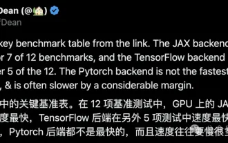 Google is ecstatic: JAX performance surpasses Pytorch and TensorFlow! It may become the fastest choice for GPU inference training
Apr 01, 2024 pm 07:46 PM
The performance of JAX, promoted by Google, has surpassed that of Pytorch and TensorFlow in recent benchmark tests, ranking first in 7 indicators. And the test was not done on the TPU with the best JAX performance. Although among developers, Pytorch is still more popular than Tensorflow. But in the future, perhaps more large models will be trained and run based on the JAX platform. Models Recently, the Keras team benchmarked three backends (TensorFlow, JAX, PyTorch) with the native PyTorch implementation and Keras2 with TensorFlow. First, they select a set of mainstream
 Slow Cellular Data Internet Speeds on iPhone: Fixes
May 03, 2024 pm 09:01 PM
Facing lag, slow mobile data connection on iPhone? Typically, the strength of cellular internet on your phone depends on several factors such as region, cellular network type, roaming type, etc. There are some things you can do to get a faster, more reliable cellular Internet connection. Fix 1 – Force Restart iPhone Sometimes, force restarting your device just resets a lot of things, including the cellular connection. Step 1 – Just press the volume up key once and release. Next, press the Volume Down key and release it again. Step 2 – The next part of the process is to hold the button on the right side. Let the iPhone finish restarting. Enable cellular data and check network speed. Check again Fix 2 – Change data mode While 5G offers better network speeds, it works better when the signal is weaker
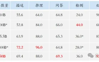 The vitality of super intelligence awakens! But with the arrival of self-updating AI, mothers no longer have to worry about data bottlenecks
Apr 29, 2024 pm 06:55 PM
I cry to death. The world is madly building big models. The data on the Internet is not enough. It is not enough at all. The training model looks like "The Hunger Games", and AI researchers around the world are worrying about how to feed these data voracious eaters. This problem is particularly prominent in multi-modal tasks. At a time when nothing could be done, a start-up team from the Department of Renmin University of China used its own new model to become the first in China to make "model-generated data feed itself" a reality. Moreover, it is a two-pronged approach on the understanding side and the generation side. Both sides can generate high-quality, multi-modal new data and provide data feedback to the model itself. What is a model? Awaker 1.0, a large multi-modal model that just appeared on the Zhongguancun Forum. Who is the team? Sophon engine. Founded by Gao Yizhao, a doctoral student at Renmin University’s Hillhouse School of Artificial Intelligence.
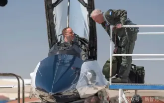 The U.S. Air Force showcases its first AI fighter jet with high profile! The minister personally conducted the test drive without interfering during the whole process, and 100,000 lines of code were tested for 21 times.
May 07, 2024 pm 05:00 PM
Recently, the military circle has been overwhelmed by the news: US military fighter jets can now complete fully automatic air combat using AI. Yes, just recently, the US military’s AI fighter jet was made public for the first time and the mystery was unveiled. The full name of this fighter is the Variable Stability Simulator Test Aircraft (VISTA). It was personally flown by the Secretary of the US Air Force to simulate a one-on-one air battle. On May 2, U.S. Air Force Secretary Frank Kendall took off in an X-62AVISTA at Edwards Air Force Base. Note that during the one-hour flight, all flight actions were completed autonomously by AI! Kendall said - "For the past few decades, we have been thinking about the unlimited potential of autonomous air-to-air combat, but it has always seemed out of reach." However now,
 The first robot to autonomously complete human tasks appears, with five fingers that are flexible and fast, and large models support virtual space training
Mar 11, 2024 pm 12:10 PM
This week, FigureAI, a robotics company invested by OpenAI, Microsoft, Bezos, and Nvidia, announced that it has received nearly $700 million in financing and plans to develop a humanoid robot that can walk independently within the next year. And Tesla’s Optimus Prime has repeatedly received good news. No one doubts that this year will be the year when humanoid robots explode. SanctuaryAI, a Canadian-based robotics company, recently released a new humanoid robot, Phoenix. Officials claim that it can complete many tasks autonomously at the same speed as humans. Pheonix, the world's first robot that can autonomously complete tasks at human speeds, can gently grab, move and elegantly place each object to its left and right sides. It can autonomously identify objects


