A brief analysis of calculating GMAC and GFLOPS
GMAC stands for "Giga Multiply-Add Operations per Second" and is an indicator used to measure the computational efficiency of deep learning models. This metric represents the computational speed of the model in terms of one billion multiplication and addition operations per second.

The multiply-accumulate (MAC) operation is fundamental in many mathematical calculations, including matrix multiplication, convolution, and other tensor operations commonly used in deep learning. Each MAC operation involves multiplying two numbers and adding the result to an accumulator.
The GMAC indicator can be calculated using the following formula:
<code>GMAC =(乘法累加运算次数)/(10⁹)</code>
The number of multiply-add operations is usually determined by analyzing the network architecture and the dimensions of the model parameters, such as weights and biases.
With the GMAC metric, researchers and practitioners can make informed decisions about model selection, hardware requirements, and optimization strategies for efficient and effective deep learning computations.
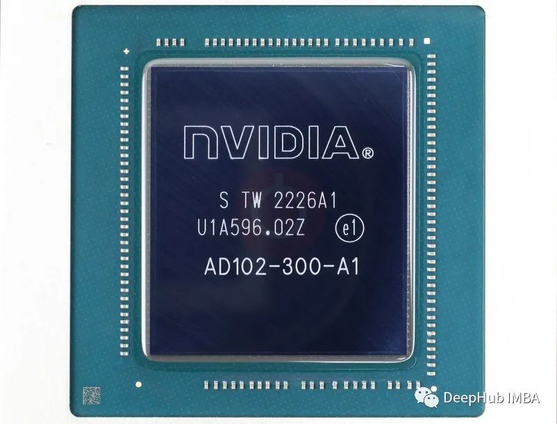
GFLOPS is a measure of computing performance of a computer system or a specific operation, representing one billion floating-point operations per second. It is the number of floating point operations per second, expressed in billions (giga).
Floating point arithmetic refers to performing arithmetic calculations on real numbers represented in IEEE 754 floating point format. These operations typically include addition, subtraction, multiplication, division, and other mathematical operations.
GFLOPS is commonly used in high-performance computing (HPC) and benchmarking, especially in areas that require heavy computational tasks, such as scientific simulations, data analysis, and deep learning.
Calculate the GFLOPS formula as follows:
<code>GFLOPS =(浮点运算次数)/(以秒为单位的运行时间)/ (10⁹)</code>
GFLOPS is an effective measure of the computing power of different computer systems, processors, or specific operations. It helps evaluate the speed and efficiency of hardware or algorithms that perform floating point calculations. GFLOPS is a measure of theoretical peak performance and may not reflect the actual performance achieved in real-world scenarios because it does not take into account factors such as memory access, parallelization, and other system limitations.
The relationship between GMAC and GFLOPS
<code>1 GFLOP = 2 GMAC</code>
If we want to calculate these two indicators, it will be more troublesome to write the code manually, but Python already has a ready-made library for us to use:
ptflops library can calculate GMAC and GFLOPs
<code>pip install ptflops</code>
It is also very simple to use:
<code>import torchvision.models as models import torch from ptflops import get_model_complexity_info import re #Model thats already available net = models.densenet161() macs, params = get_model_complexity_info(net, (3, 224, 224), as_strings=True, print_per_layer_stat=True, verbose=True) # Extract the numerical value flops = eval(re.findall(r'([\d.]+)', macs)[0])*2 # Extract the unit flops_unit = re.findall(r'([A-Za-z]+)', macs)[0][0] print('Computational complexity: {:</code>The results are as follows:
<code>Computational complexity: 7.82 GMac Computational complexity: 15.64 GFlops Number of parameters: 28.68 M</code>
We can customize a model to take a look Is the result correct?
<code>import os import torch from torch import nn class NeuralNetwork(nn.Module): def __init__(self): super().__init__() self.flatten = nn.Flatten() self.linear_relu_stack = nn.Sequential( nn.Linear(28*28, 512), nn.ReLU(), nn.Linear(512, 512), nn.ReLU(), nn.Linear(512, 10),) def forward(self, x): x = self.flatten(x) logits = self.linear_relu_stack(x) return logits custom_net = NeuralNetwork() macs, params = get_model_complexity_info(custom_net, (28, 28), as_strings=True, print_per_layer_stat=True, verbose=True) # Extract the numerical value flops = eval(re.findall(r'([\d.]+)', macs)[0])*2 # Extract the unit flops_unit = re.findall(r'([A-Za-z]+)', macs)[0][0] print('Computational complexity: {:</code>The result is as follows:
<code>Computational complexity: 670.73 KMac Computational complexity: 1341.46 KFlops Number of parameters: 669.71 k</code>
For the convenience of demonstration, we only write the fully connected layer code to manually calculate GMAC. Iterating over the model weight parameters and calculating the shape of the number of multiplication and addition operations depends on the weight parameters, which is the key to calculating GMAC. The formula for calculating the fully connected layer weight required by GMAC is 2 x (input dimension x output dimension). The total GMAC value is obtained by multiplying and accumulating the shapes of the weight parameters of each linear layer, a process based on the structure of the model.
<code>import torch import torch.nn as nn def compute_gmac(model): gmac_count = 0 for param in model.parameters(): shape = param.shape if len(shape) == 2:# 全连接层的权重 gmac_count += shape[0] * shape[1] * 2 gmac_count = gmac_count / 1e9# 转换为十亿为单位 return gmac_count</code>
According to the model given above, the result of calculating GMAC is as follows:
<code>0.66972288</code>
Since the result of GMAC is in billions, it is not much different from the result we calculated using the class library above . Finally, calculating the GMAC of convolution is a little complicated. The formula is ((input channel x convolution kernel height x convolution kernel width) x output channel) x 2. Here is a simple code, which may not be completely correct. Reference
<code>def compute_gmac(model): gmac_count = 0 for param in model.parameters(): shape = param.shape if len(shape) == 2:# 全连接层的权重 gmac_count += shape[0] * shape[1] * 2 elif len(shape) == 4:# 卷积层的权重 gmac_count += shape[0] * shape[1] * shape[2] * shape[3] * 2 gmac_count = gmac_count / 1e9# 转换为十亿为单位 return gmac_count</code>
The above is the detailed content of A brief analysis of calculating GMAC and GFLOPS. For more information, please follow other related articles on the PHP Chinese website!

Hot AI Tools

Undresser.AI Undress
AI-powered app for creating realistic nude photos

AI Clothes Remover
Online AI tool for removing clothes from photos.

Undress AI Tool
Undress images for free

Clothoff.io
AI clothes remover

AI Hentai Generator
Generate AI Hentai for free.

Hot Article

Hot Tools

Notepad++7.3.1
Easy-to-use and free code editor

SublimeText3 Chinese version
Chinese version, very easy to use

Zend Studio 13.0.1
Powerful PHP integrated development environment

Dreamweaver CS6
Visual web development tools

SublimeText3 Mac version
God-level code editing software (SublimeText3)

Hot Topics
 Methods and steps for using BERT for sentiment analysis in Python
Jan 22, 2024 pm 04:24 PM
BERT is a pre-trained deep learning language model proposed by Google in 2018. The full name is BidirectionalEncoderRepresentationsfromTransformers, which is based on the Transformer architecture and has the characteristics of bidirectional encoding. Compared with traditional one-way coding models, BERT can consider contextual information at the same time when processing text, so it performs well in natural language processing tasks. Its bidirectionality enables BERT to better understand the semantic relationships in sentences, thereby improving the expressive ability of the model. Through pre-training and fine-tuning methods, BERT can be used for various natural language processing tasks, such as sentiment analysis, naming
 Analysis of commonly used AI activation functions: deep learning practice of Sigmoid, Tanh, ReLU and Softmax
Dec 28, 2023 pm 11:35 PM
Activation functions play a crucial role in deep learning. They can introduce nonlinear characteristics into neural networks, allowing the network to better learn and simulate complex input-output relationships. The correct selection and use of activation functions has an important impact on the performance and training results of neural networks. This article will introduce four commonly used activation functions: Sigmoid, Tanh, ReLU and Softmax, starting from the introduction, usage scenarios, advantages, disadvantages and optimization solutions. Dimensions are discussed to provide you with a comprehensive understanding of activation functions. 1. Sigmoid function Introduction to SIgmoid function formula: The Sigmoid function is a commonly used nonlinear function that can map any real number to between 0 and 1. It is usually used to unify the
 Beyond ORB-SLAM3! SL-SLAM: Low light, severe jitter and weak texture scenes are all handled
May 30, 2024 am 09:35 AM
Written previously, today we discuss how deep learning technology can improve the performance of vision-based SLAM (simultaneous localization and mapping) in complex environments. By combining deep feature extraction and depth matching methods, here we introduce a versatile hybrid visual SLAM system designed to improve adaptation in challenging scenarios such as low-light conditions, dynamic lighting, weakly textured areas, and severe jitter. sex. Our system supports multiple modes, including extended monocular, stereo, monocular-inertial, and stereo-inertial configurations. In addition, it also analyzes how to combine visual SLAM with deep learning methods to inspire other research. Through extensive experiments on public datasets and self-sampled data, we demonstrate the superiority of SL-SLAM in terms of positioning accuracy and tracking robustness.
 Latent space embedding: explanation and demonstration
Jan 22, 2024 pm 05:30 PM
Latent Space Embedding (LatentSpaceEmbedding) is the process of mapping high-dimensional data to low-dimensional space. In the field of machine learning and deep learning, latent space embedding is usually a neural network model that maps high-dimensional input data into a set of low-dimensional vector representations. This set of vectors is often called "latent vectors" or "latent encodings". The purpose of latent space embedding is to capture important features in the data and represent them into a more concise and understandable form. Through latent space embedding, we can perform operations such as visualizing, classifying, and clustering data in low-dimensional space to better understand and utilize the data. Latent space embedding has wide applications in many fields, such as image generation, feature extraction, dimensionality reduction, etc. Latent space embedding is the main
 Understand in one article: the connections and differences between AI, machine learning and deep learning
Mar 02, 2024 am 11:19 AM
In today's wave of rapid technological changes, Artificial Intelligence (AI), Machine Learning (ML) and Deep Learning (DL) are like bright stars, leading the new wave of information technology. These three words frequently appear in various cutting-edge discussions and practical applications, but for many explorers who are new to this field, their specific meanings and their internal connections may still be shrouded in mystery. So let's take a look at this picture first. It can be seen that there is a close correlation and progressive relationship between deep learning, machine learning and artificial intelligence. Deep learning is a specific field of machine learning, and machine learning
 Super strong! Top 10 deep learning algorithms!
Mar 15, 2024 pm 03:46 PM
Almost 20 years have passed since the concept of deep learning was proposed in 2006. Deep learning, as a revolution in the field of artificial intelligence, has spawned many influential algorithms. So, what do you think are the top 10 algorithms for deep learning? The following are the top algorithms for deep learning in my opinion. They all occupy an important position in terms of innovation, application value and influence. 1. Deep neural network (DNN) background: Deep neural network (DNN), also called multi-layer perceptron, is the most common deep learning algorithm. When it was first invented, it was questioned due to the computing power bottleneck. Until recent years, computing power, The breakthrough came with the explosion of data. DNN is a neural network model that contains multiple hidden layers. In this model, each layer passes input to the next layer and
 How to use CNN and Transformer hybrid models to improve performance
Jan 24, 2024 am 10:33 AM
Convolutional Neural Network (CNN) and Transformer are two different deep learning models that have shown excellent performance on different tasks. CNN is mainly used for computer vision tasks such as image classification, target detection and image segmentation. It extracts local features on the image through convolution operations, and performs feature dimensionality reduction and spatial invariance through pooling operations. In contrast, Transformer is mainly used for natural language processing (NLP) tasks such as machine translation, text classification, and speech recognition. It uses a self-attention mechanism to model dependencies in sequences, avoiding the sequential computation in traditional recurrent neural networks. Although these two models are used for different tasks, they have similarities in sequence modeling, so
 Improved RMSprop algorithm
Jan 22, 2024 pm 05:18 PM
RMSprop is a widely used optimizer for updating the weights of neural networks. It was proposed by Geoffrey Hinton et al. in 2012 and is the predecessor of the Adam optimizer. The emergence of the RMSprop optimizer is mainly to solve some problems encountered in the SGD gradient descent algorithm, such as gradient disappearance and gradient explosion. By using the RMSprop optimizer, the learning rate can be effectively adjusted and the weights adaptively updated, thereby improving the training effect of the deep learning model. The core idea of the RMSprop optimizer is to perform a weighted average of gradients so that gradients at different time steps have different effects on weight updates. Specifically, RMSprop calculates the square of each parameter


