

How to get the name of the current worksheet in Excel

Excel does not provide a built-in formula to immediately return the name of the active Excel worksheet. In some scenarios, you may need to dynamically populate values into the active worksheet in an Excel file. For example, if the table name on a worksheet must be the name of the worksheet itself, and if you hardcode the table name and later change the worksheet name, you must also change the table name manually. However, if the table's name is populated dynamically, such as using a formula, then if the sheet name changes, the table's name will also change automatically.
While the requirement most likely exists, there is no direct formula for extracting the name of the active worksheet, as stated previously. We do have some combination of formulas that will allow you to successfully extract the name of the active sheet. Read on to find out how!
Section 1: How to get the name of the current worksheet using a combination of Right, Cell, Find, and Len functions
Section 1.1: Complete formula
The first step is to make sure you have saved the Excel worksheet. If you haven't saved the Excel document yet, please save it first, otherwise this formula will not work.
To save a document, you just need to press the CTRL S keys simultaneously, navigate to the location where you want to save the document, give the file a name, and finally save.
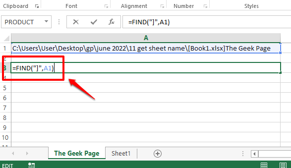
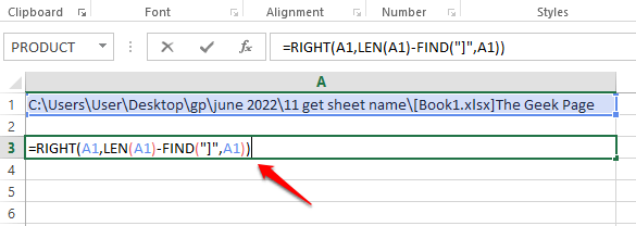
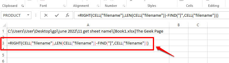
Step 1: After saving the Excel document, just double-click on any cell. Once in edit mode, copy and paste the following formula, and then press Enter.
=RIGHT(CELL("文件名"),LEN(CELL("文件名"))-FIND("]",CELL("文件名")))Note: Don’t worry about seeing the length of the formula, in the section below, we have explained the formula in detail.
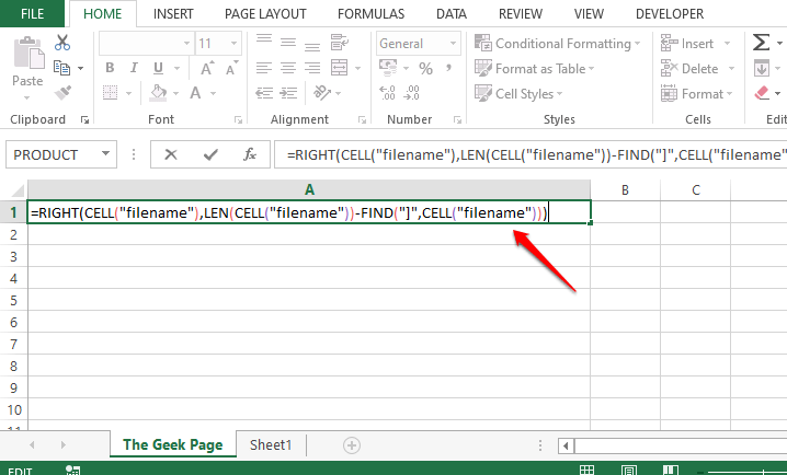
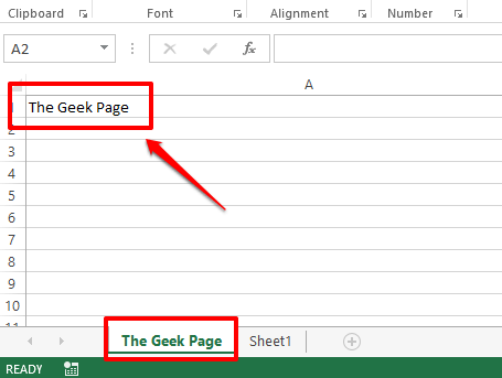
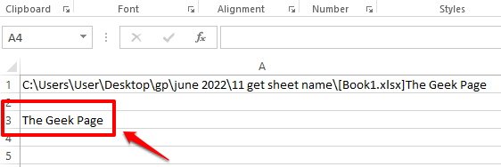
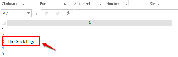
Step 2: Once you press the Enter key, you can see the name of the current worksheet, below In the example, the worksheet name is The Geek Page, which is returned successfully on the cell where the formula is entered. Yes, it's simple and we agree. But if you want to know how this formula works, you can refer to the section below.
Section 1.2: Formula Description
In this section, let us take out the lengthy formula from the above section, Split it up and find out what's really going on and how it successfully returns the name of the current worksheet.
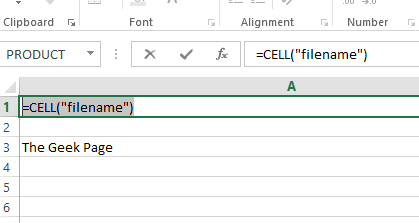
Step 1: The first part of the formula is =CELL(“filename”). cellThe function only accepts one parameter. It returns the full address of the cell, including the worksheet's file location and the current worksheet name.
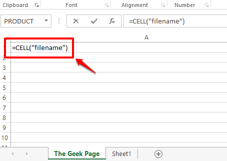
Step 2: If you look at the screenshot below, if you press the Enter key, you will get the entire file name, including the last name of the current worksheet.
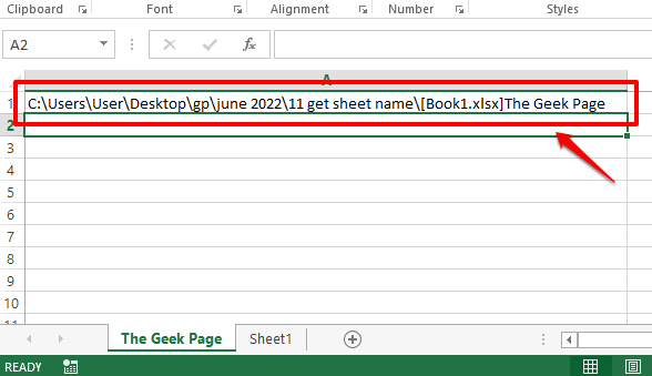
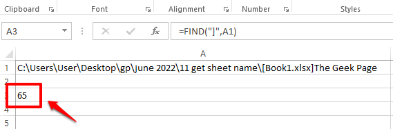
Step 3: As you can see, the worksheet name is at the end of the file name. To be precise, anything after the right square bracket ] is jobtablename. So, let us use the FIND function to find the index value of the square bracket character. After we find that index, let's find all the characters that follow it, which is essentially the worksheet name. The
FIND function takes two parameters, one is the character whose index is to be found, and the second is the string on which the search is to be performed. So, in this particular case, our FIND function would look like this.
=查找(“]”,A1)
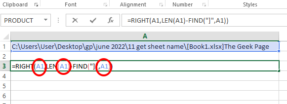
A1 is the cell ID of the cell containing the file name we found using the CELL function. If your filename is in a different cell, you should provide that cell id instead of A1.
Step 4: FINDThe function returns the value 65. This means that the right bracket is at position 65. So we need to extract everything after the 65th bit from the file name, that is, everything after the closing square bracket.
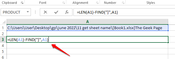
Step 5: To extract everything after the 65th bit, we first need to know how many characters to extract after the 65th bit. To make it easier, we need to know how many characters our current worksheet name is. For this, let's use the LEN function. The functions are as follows.
=LEN(A1)-FIND("]",A1)上面的公式只返回工作表名称的长度。首先使用LEN(A1)计算文件名的长度,然后减去文件名的长度直到右方括号,即 65。
第6步:上面的公式返回13,这是当前工作表名称The Geek Page的长度。
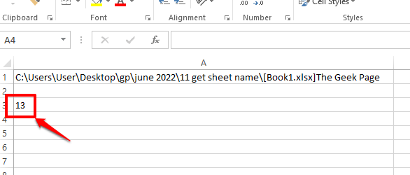
第 7 步:所以我们现在有了源字符串,它是完整的文件名,我们知道当前工作表名称有 13 个字符,并且位于文件名的末尾。因此,如果我们从文件名的最右边提取 13 个字符,我们将得到当前工作表名称。
现在,让我们直接使用RIGHT函数提取工作表名称。RIGHT函数如下。
=RIGHT(A1, LEN(A1)-查找("]",A1))RIGHT函数有2 个参数,一个是要从中提取子字符串的字符串,第二个是需要从父字符串右侧提取的字符数。
现在,下面的屏幕截图会详细告诉您这一点。RIGHT函数接受文件名和当前工作表的长度。因此,从文件名中,RIGHT字符串将从字符串的最右侧提取工作表名称,根据上述步骤计算,该名称为 13 个字符。
第8步:你去!现在已成功提取活动工作表的名称!
第九步:名字解压成功,但是有一个小依赖。我们的公式依赖于定义CELL函数的单元格。我们继续提到A1。有一件事是,我们可能不希望文档中包含完整的文件名,因此将它放在文档中可能会带来巨大的不便。另一件事是,如果我们删除它,我们的公式将不再起作用,因为它具有依赖关系。因此,让我们删除依赖项。
为此,双击定义 CELL 函数的单元格并复制整个公式。您可以通过选择公式,然后同时按下CTRL + C键来复制公式。
第 10 步:现在在我们的RIGHT公式中,将 A1 替换为您在第 9 步中复制的 CELL 函数。RIGHT 公式中出现了 3 次 A1,因此必须替换所有 3 次。
第 11 步:下面的屏幕截图显示了替换后的 RIGHT 公式应该是什么样子。
第12步:如果你按回车键或点击其他地方,你可以看到当前工作表名称被成功提取。此外,由于不再存在依赖关系,您可以删除A1单元格。享受!
第 2 节:如何使用 Mid、Cell 和 Find 函数的组合获取当前工作表的名称
这是另一个公式组合,您可以使用它找到活动工作表的名称。在这个公式中,我们没有使用RIGHT函数,而是使用了MID函数。公式如下。
=MID(CELL("文件名"),FIND("]",CELL("文件名"))+1,255)在 Excel 文档中,双击任意单元格并简单地复制粘贴上述公式并按Enter键。您将获得在您输入公式的单元格上返回的活动工作表的名称。
注意:如果我们给出子字符串的起始位置及其长度, MID函数会从主字符串返回子字符串。
另请注意,即使要使此公式起作用,您也应该首先将文档保存在某个地方,否则您将收到Value 错误。
即使 Excel 中没有直接的公式,您可以使用它直接获取活动工作表的名称,但使用上述任一公式组合,您都可以获得所需的结果。
The above is the detailed content of How to get the name of the current worksheet in Excel. For more information, please follow other related articles on the PHP Chinese website!

Hot AI Tools

Undresser.AI Undress
AI-powered app for creating realistic nude photos

AI Clothes Remover
Online AI tool for removing clothes from photos.

Undress AI Tool
Undress images for free

Clothoff.io
AI clothes remover

AI Hentai Generator
Generate AI Hentai for free.

Hot Article
Hot Tools

Notepad++7.3.1
Easy-to-use and free code editor

SublimeText3 Chinese version
Chinese version, very easy to use

Zend Studio 13.0.1
Powerful PHP integrated development environment

Dreamweaver CS6
Visual web development tools

SublimeText3 Mac version
God-level code editing software (SublimeText3)
Hot Topics
 1378
1378
 52
52

 Excel found a problem with one or more formula references: How to fix it
Apr 17, 2023 pm 06:58 PM
Excel found a problem with one or more formula references: How to fix it
Apr 17, 2023 pm 06:58 PM
Use an Error Checking Tool One of the quickest ways to find errors with your Excel spreadsheet is to use an error checking tool. If the tool finds any errors, you can correct them and try saving the file again. However, the tool may not find all types of errors. If the error checking tool doesn't find any errors or fixing them doesn't solve the problem, then you need to try one of the other fixes below. To use the error checking tool in Excel: select the Formulas tab. Click the Error Checking tool. When an error is found, information about the cause of the error will appear in the tool. If it's not needed, fix the error or delete the formula causing the problem. In the Error Checking Tool, click Next to view the next error and repeat the process. When not
 How to set the print area in Google Sheets?
May 08, 2023 pm 01:28 PM
How to set the print area in Google Sheets?
May 08, 2023 pm 01:28 PM
How to Set GoogleSheets Print Area in Print Preview Google Sheets allows you to print spreadsheets with three different print areas. You can choose to print the entire spreadsheet, including each individual worksheet you create. Alternatively, you can choose to print a single worksheet. Finally, you can only print a portion of the cells you select. This is the smallest print area you can create since you could theoretically select individual cells for printing. The easiest way to set it up is to use the built-in Google Sheets print preview menu. You can view this content using Google Sheets in a web browser on your PC, Mac, or Chromebook. To set up Google
 How to embed a PDF document in an Excel worksheet
May 28, 2023 am 09:17 AM
How to embed a PDF document in an Excel worksheet
May 28, 2023 am 09:17 AM
It is usually necessary to insert PDF documents into Excel worksheets. Just like a company's project list, we can instantly append text and character data to Excel cells. But what if you want to attach the solution design for a specific project to its corresponding data row? Well, people often stop and think. Sometimes thinking doesn't work either because the solution isn't simple. Dig deeper into this article to learn how to easily insert multiple PDF documents into an Excel worksheet, along with very specific rows of data. Example Scenario In the example shown in this article, we have a column called ProductCategory that lists a project name in each cell. Another column ProductSpeci
 What should I do if there are too many different cell formats that cannot be copied?
Mar 02, 2023 pm 02:46 PM
What should I do if there are too many different cell formats that cannot be copied?
Mar 02, 2023 pm 02:46 PM
Solution to the problem that there are too many different cell formats that cannot be copied: 1. Open the EXCEL document, and then enter the content of different formats in several cells; 2. Find the "Format Painter" button in the upper left corner of the Excel page, and then click " "Format Painter" option; 3. Click the left mouse button to set the format to be consistent.
 How to remove commas from numeric and text values in Excel
Apr 17, 2023 pm 09:01 PM
How to remove commas from numeric and text values in Excel
Apr 17, 2023 pm 09:01 PM
On numeric values, on text strings, using commas in the wrong places can really get annoying, even for the biggest Excel geeks. You may even know how to get rid of commas, but the method you know may be time-consuming for you. Well, no matter what your problem is, if it is related to a comma in the wrong place in your Excel worksheet, we can tell you one thing, all your problems will be solved today, right here! Dig deeper into this article to learn how to easily remove commas from numbers and text values in the simplest steps possible. Hope you enjoy reading. Oh, and don’t forget to tell us which method catches your eye the most! Section 1: How to Remove Commas from Numerical Values When a numerical value contains a comma, there are two possible situations:
 How to find and delete merged cells in Excel
Apr 20, 2023 pm 11:52 PM
How to find and delete merged cells in Excel
Apr 20, 2023 pm 11:52 PM
How to Find Merged Cells in Excel on Windows Before you can delete merged cells from your data, you need to find them all. It's easy to do this using Excel's Find and Replace tool. Find merged cells in Excel: Highlight the cells where you want to find merged cells. To select all cells, click in an empty space in the upper left corner of the spreadsheet or press Ctrl+A. Click the Home tab. Click the Find and Select icon. Select Find. Click the Options button. At the end of the FindWhat settings, click Format. Under the Alignment tab, click Merge Cells. It should contain a check mark rather than a line. Click OK to confirm the format
 How to prevent Excel from removing leading zeros
Feb 29, 2024 am 10:00 AM
How to prevent Excel from removing leading zeros
Feb 29, 2024 am 10:00 AM
Is it frustrating to automatically remove leading zeros from Excel workbooks? When you enter a number into a cell, Excel often removes the leading zeros in front of the number. By default, it treats cell entries that lack explicit formatting as numeric values. Leading zeros are generally considered irrelevant in number formats and are therefore omitted. Additionally, leading zeros can cause problems in certain numerical operations. Therefore, zeros are automatically removed. This article will teach you how to retain leading zeros in Excel to ensure that the entered numeric data such as account numbers, zip codes, phone numbers, etc. are in the correct format. In Excel, how to allow numbers to have zeros in front of them? You can preserve leading zeros of numbers in an Excel workbook, there are several methods to choose from. You can set the cell by
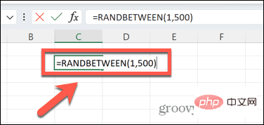 How to create a random number generator in Excel
Apr 14, 2023 am 09:46 AM
How to create a random number generator in Excel
Apr 14, 2023 am 09:46 AM
How to use RANDBETWEEN to generate random numbers in Excel If you want to generate random numbers within a specific range, the RANDBETWEEN function is a quick and easy way to do it. This allows you to generate random integers between any two values of your choice. Generate random numbers in Excel using RANDBETWEEN: Click the cell where you want the first random number to appear. Type =RANDBETWEEN(1,500) replacing "1" with the lowest random number you want to generate and "500" with