
 Technology peripherals
AI
Detailed explanation of obstacle avoidance, path planning and control technology for autonomous vehicles
Technology peripherals
AI
Detailed explanation of obstacle avoidance, path planning and control technology for autonomous vehicles
Detailed explanation of obstacle avoidance, path planning and control technology for autonomous vehicles

1 Introduction
Intelligent transportation systems address challenging autonomy and safety issues in complex environments, and therefore it attracts special attention from researchers. The main modules of the autonomous vehicle concept are perception, planning and control.
Actually, perception consists of environment modeling and localization. They rely on external and body sensors respectively. Next, planning aims to generate an optimal trajectory based on the information conveyed by the sensing results in order to reach a given destination. Finally, the control module is dedicated to tracking the generated trajectory by commanding the vehicle's actuators.
This article will introduce each module of the process for the specific situation of avoiding obstacles. The integration of these tasks in a global architecture is the main contribution of this paper. The perception module ensures that the environment is described based on an accurate grid representation. The use of Occupancy Grid Maps (OGM) is particularly convenient for obstacle avoidance, as it can identify drivable spaces and locate static and dynamic objects in the scene. The pose of the object to be avoided is then used at the path planning level, which generates trajectories and velocity profiles based on the sigmoid parameterized function and rolling horizon shown in [1]. The obtained curvature profile is considered as the reference path to guide the control module. This level provides the vehicle with the appropriate steering angle based on a lateral guidance controller that uses the center of impact (CoP) instead of the classic center of gravity. The proposed controller is based on feedforward and robust state feedback actions to reduce the impact of disturbances on lateral errors and ensure lateral stability, respectively [2].
The paper is organized as follows: Part II presents the global approach, which contains the different modules that will be implemented for obstacle avoidance. The third part introduces the dynamic object detection method based on confidence grid occupancy. Section 4 explains the obstacle avoidance algorithm based on parameterized sigmoid function and rolling horizon. Section 5 details the controller design based on feedforward coupling to robust state feedback. Section 6 describes the experimental platform and results of this experimental method. Finally, Section 7 concludes the paper.
2 Obstacle avoidance strategy
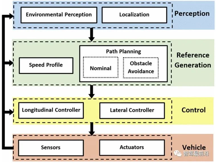
#This section introduces the title of the global obstacle avoidance strategy based on three modules, as shown in Figure 1. This section briefly introduces each level.
 Picture
Figure 1 Obstacle avoidance strategy
A. Perception Module
#Perceiving the environment correctly and effectively is mandatory for autonomous vehicles. This research mainly focuses on environment perception to extract the locations of static/dynamic objects and drivable paths based on external sensing sensors. The position of the vehicle not considered in the positioning part is considered known and reliable. One of the most common methods to extract information about roads and surrounding objects is the "Occupancy Grid" (OG). It can be used in a variety of applications such as collision avoidance, sensor fusion, target tracking, and simultaneous localization and mapping (SLAM) [3]. The basic idea of OG is to represent the environment graph as uniformly spaced fields of binary random variables, each variable representing whether there is an obstacle at that location in the environment [4]. It can be generated from a number of forms to handle noisy and uncertain sensor measurements given a known vehicle attitude. In this paper, OG is defined by the belief theory proposed by Dempster and Shafer [5][6] as it models uncertainty, imprecision and unknown parts and also allows managing conflicts in data fusion. Part 3 gives more details.
B. Reference trajectory generation module
This module is dedicated to defining the trajectory and the corresponding speed curve that the vehicle should follow. . The planner receives the drivable area and obstacle locations from the perception module. Based on this information, geometric trajectories and velocity curves can be generated. This article focuses on path planning strategies. This section aims to provide a nominal trajectory from a start point to an end point based on the perceived drivable area.
When an obstacle is detected, the second trajectory (obstacle avoidance trajectory) is calculated to ensure the safety and comfort of the autonomous vehicle passengers, and the nominal trajectory is added after avoidance . This avoidance trajectory can be obtained by local planning since it involves only a small part of the nominal trajectory. To reduce the computational cost of the trajectory generation algorithm, the rolling horizon method is adopted, as described in [1], whose work is extended in this paper, see Section IV. These trajectories (nominal and obstacle avoidance) can then be considered as references for control modules (mainly lateral controllers).
C. Control module
The control module consists of two main parts: longitudinal and lateral controllers, which ensure automatic driving control. The main focus here is on lateral controllers to handle obstacle avoidance. In fact, the appropriate steering angle is provided by the lateral controller to follow the desired path given by the reference generation module. Tracking of the desired path can be achieved by reducing two tracking errors, namely lateral error and heading error. Among the geometric and dynamic lateral guidance strategies present in the literature [7], a dynamic approach based on the Center of Collision (CoP) is adopted here [8]. The choice depends on the performance of this control method. The CoP is a geometric point located in front of the vehicle's center of gravity (CoG) that predicts lateral position errors. One can then expect better trajectory tracking. On the other hand, since the motion of the CoP is decoupled from the rear tire lateral force [9], as shown in Section V, the lateral dynamics equation becomes less complex.
2 Dynamic obstacle detection based on dynamic grid
OG is a representation that subdivides the multi-dimensional space into units. Each unit stores knowledge of its occupancy status [4]. Today, OG is heavily used as more powerful resources are available to handle its computational complexity. The construction of meshes has been applied in multiple dimensions (2D, 2.5D and 3D) [10], where each cell state is described according to a selected form. The most common is the Bayesian framework, which was first adopted by Elfes [4] and subsequently underwent many extensions to become the famous Bayesian Occupancy Filter (BOF) [11]. Other works propose a formalism based on Dempster-Shafer theory, also known as evidence theory, which is described subsequently.
A. Using belief theory
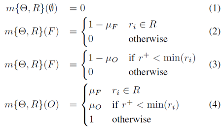
#Summary to probability theory, belief theory provides sufficient coverage of data and source defects representation and therefore suitable for perception in ITS. It provides a wide range of fusion operators that can handle these properties depending on the application. Some research on building OG using the Belief framework can be found in [12], [13]. This work originates from the research of [13], which proposed a method for moving object detection and drivable space determination based on the resulting conflicts. To this end, an identification frame is defined to include the status of a cell that is considered free (F) or occupied (O). The recognition box is Ω={F, O}. The reference power set framework contains all possible combinations of the following assumptions: 2Ω= {∅,F,O,{F,O}}. In order to express the belief in each state, the mass function m(.) represents the conflict m(∅), the free state m(F), the occupied state m(O) and the unknown state m({F,O}) respectively.
B. Sensor Model
#Basically, the sensor model is how to calculate the quality function of the state corresponding to the metric . In our application, the sensor to be used is a 3D multi-echo LIDAR (see Section VI). The input data will include a range ri based on a point pi and an angle θi. From this data set, a scanning grid (SG) in polar coordinates is constructed. Each row of SG corresponds to an angular sector Θ=[θ-, θ] defined in RxΘ. The range of the cell is R=[r-,r] which means that each cell is defined by a pair of masses m{Θ,R}. The mass A∈Ω corresponding to each proposition is found here [13]:
 Picture
where μF and μO correspond respectively The probability of false alarms and missed detections due to the sensor. For simplicity, these mass functions, m(O), m(F) and m(Θ), will be illustrated.
 Picture
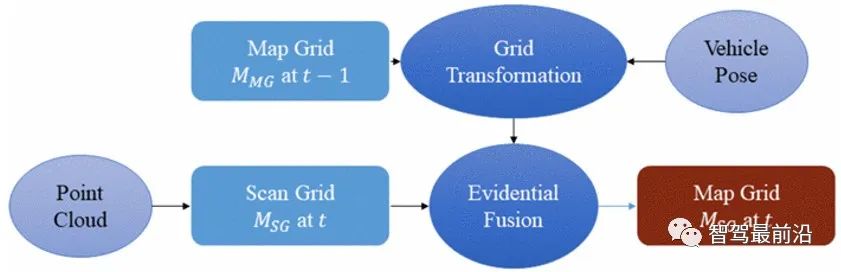
Figure 2 Map grid (MG) structure
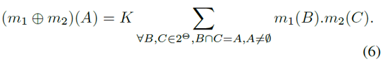
Figure 2 shows the process of building and updating the MG using the sensor point cloud provided at time t. This update is done based on multi-grid evidence fusion. This is the most interesting part of the process, as it allows time to update the map grid and evaluate unit status. Among the various operators of belief theory, the Dempster-Shafer combination rule is used:

where mmG,t and mmG,t-1 respectively represents the quality function of the map grid and scanned grid at time t. The operator is defined as:
where
produces The result of mmG,t(A) defines the state of each cell, which depends on the previous state and the new metric. It was found that the mass produced according to each state is as follows [13]:
Basically, this property shows the dissonance between t-1 and t. Inconsistency occurs when a unit changes from Free to Occupied or vice versa. Therefore, the detection of conflicts can lead to the evaluation of dynamic cells. Conflicts allow marking occupied cells that change their status based on two conflict types:
where,
The fusion process normalizes the state quality by the total collision, but considers using this information to mark mobile units that define dynamic objects. Each detected pose is then used as input for trajectory generation in the next section.
4 Trajectory generation
This section is dedicated to path planning, that is, creating a geometric trajectory (following coordinate points) Ai(xi,yi) . Since this paper aims to verify the feasibility of the proposed avoidance architecture, the speed curve and the associated longitudinal control are not considered. As mentioned in Section 2, the path planning module has two goals: to generate a global nominal trajectory based on the origin and arrival points, and to generate a local trajectory to avoid detecting obstacles. Here, the focus is on the generation of avoidance trajectories. This avoidance trajectory must comply with safety standards, in particular the longitudinal and lateral distances to obstacles. These distances can be equal, creating a circular safety zone around the obstacle, as recently suggested in [1]. This paper proposes a generalization of the method by considering the overall situation where horizontal and vertical security standards are different.
In order to obtain the geometric form of the trajectory, there are several mathematical methods based on functions such as clothoid curves, Bezier curves or splines [14], [15]. An exhaustive review of all these geometric methods is given in [16]. These methods have interesting characteristics (smoothness, selection of the best trajectory among a set of candidates, etc.), but they can be computationally expensive. Among them, the sigmoid function represents a fair trade-off between smoothness and computational cost. The approach considered recommends using this mathematical method in conjunction with a native Horizon scheduler to reduce computational costs. The advantages of this planning approach are discussed extensively in [1]. This local planner considers information about detected obstacles from the occupancy grid to define appropriate smooth avoidance maneuvers and return to the nominal trajectory.
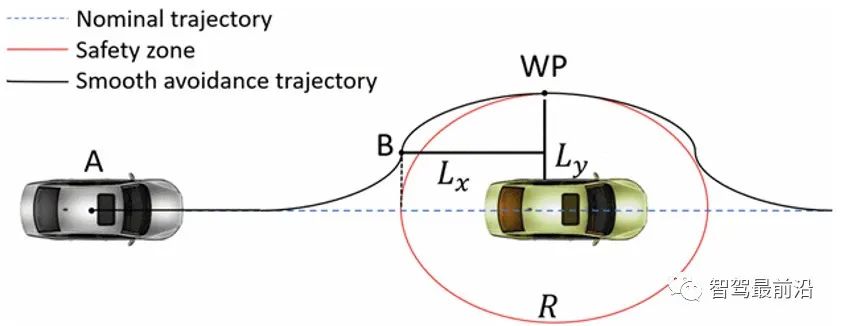
A. Geometric Avoidance
Figure 3 shows different trajectories: nominal trajectory, safe zone and The final smooth avoidance trajectory. Safety zone definition R is the first step after detecting an obstacle. This area is not navigable to avoid collisions due to proximity with obstacles. The semi-major and semi-minor axes of the Lx and Ly ellipses, respectively, are the safety criteria that define the area. Once defined, avoidance trajectories can be designed. To ensure passenger comfort, features based on the S shape were chosen. In Figure 3, A refers to the starting point (i.e. the center of gravity of the ego vehicle), B is the buckling point of the sigmoid, and WP is the starting point to be reached. The smoothness C() can be adjusted so that the avoidance trajectory can be defined as Repeat the entire process (determine the safe area and calculate the sigmoid function-based waypoint) for each horizontal vector sample.
Figure 3 Trajectory Planning
In order to reduce the computational cost of the algorithm, a local planner is used. It does not follow the entire obstacle avoidance trajectory, but is divided into several parts. Local trajectories are computed at each sample at this discrete level, reducing computational cost and making the algorithm robust to dynamic obstacles. Two parameters can be parameterized: sample size and horizontal length. The last one depends on the equipped perception sensors (hardware constraints) and vehicle speed (rolling horizon). Sample steps represent the subdivision of the trajectory into local segments. The entire principle is summarized in Figure 4.
PictureFigure 4 Horizon Planning
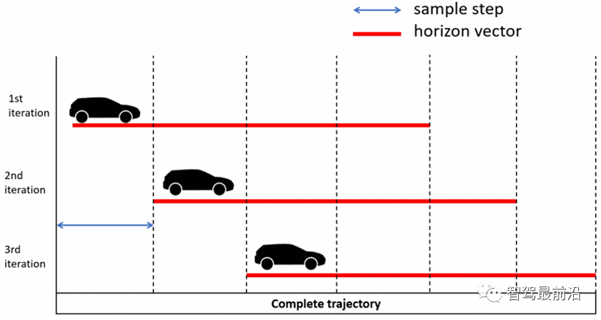
When the vehicle reaches the next sampling step, the local horizon line will be calculated again. As can be seen, there is a common part between the two iterations that allows the algorithm to handle dynamic obstacles. As with the discrete time domain, the choice of sample size requires a trade-off between accuracy and computational cost. The algorithm iterates until the horizon vector reaches the end of the complete trajectory, i.e. when the perception sensors cover all subdivisions of the trajectory. This geometric trajectory is the input to the guidance control stage.
5 Controller Design
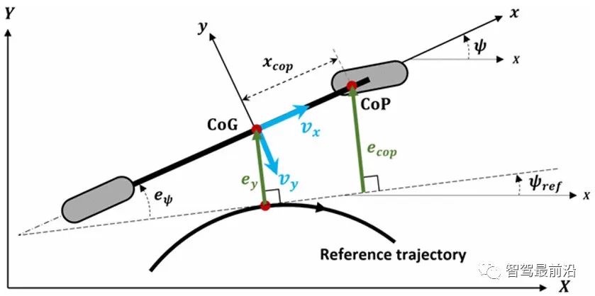
This section describes the lateral controller design used in the control module shown in Figure 1. Lateral guidance aims to reduce two types of errors, namely lateral error, the distance between the vehicle's CoG and the reference trajectory, and heading error, the distance between the vehicle's longitudinal axis and the reference trajectory, as shown in Figure 5:
 Picture
Figure 5 Lateral and heading error
Here, instead of the classic CoG lateral error ey, It is recommended to use the lateral error when the CoP is defined as [9]:

The distance between CoP and CoG xcop depends only on the vehicle configuration:
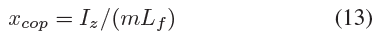
where m and Iz are the vehicle mass and yaw inertia, and lf is the distance between the CoG and the front axle. It can be seen from (12) that the CoP lateral error ecop is higher than the lateral error ey in Figure 5. This way, lateral position errors can be expected and better trajectory tracking can be expected. In contrast to classic controllers based on CoG (Center of Gravity), here the Center of Impact (CoP) is used as a geometric point on the vehicle. The main advantage of the CoP is the reduced complexity of the lateral dynamics equations, since the rear tire lateral forces do not affect the motion of the CoP [9].
Based on the planar bicycle model [17] and using tracking errors (11) and (12), the tracking error model used to design the CoP lateral navigation controller is:

where the state vector 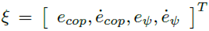 , δf is the front wheel angle,
  contains the expectation as a disturbance term Yaw angular velocity and yaw angular acceleration.
 Picture


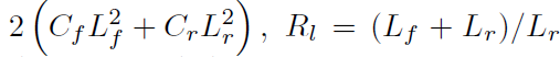
##Lr is the distance between CoG and the rear axle, Cf and Cr are the front and rear tire cornering stiffnesses. Note that Cr is not in the second row of Ac. Therefore, using CoP can reduce the number of uncertain parameters.
The lateral controller calculates appropriate δf in order to ensure that the state vector error converges close to zero. Furthermore, since the dynamics of the tracking error model are affected by wref, the controller must also ensure a level of attenuation of its influence. To achieve these goals, a lateral controller consisting of feedforward coupling to robust state feedback is proposed [2]:
 Picture
LFF and KFB are feedforward and robust feedback gains respectively. Feedforward actions aim to partially eliminate the effects of vector wref. The benefit of CoP is that the feedforward obtained does not require knowledge of Cr. The state feedback action ensures exponential convergence of the error vector towards zero and attenuates the influence of the vector wref. This robust control problem can be expressed using linear matrix inequalities (LMI) as shown in [2].
6 Experimental results
A. Experimental settings
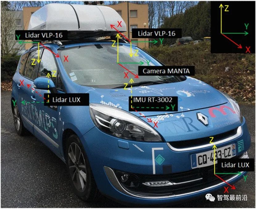
The experimental platform ARTEMIPS is an automatic test vehicle equipped with multiple sensors: high-precision IMU (Inertial Measurement Unit) RT-3002 using DGPS technology, 2 IBEO LUX 2D 4-layer laser scanners, 2 VLPs -16 Velodyne3D laser scanner and high-range camera MANTA-G125 (see Figure 6)). RT-3002 is used as a reference sensor for position, velocity, acceleration and direction measurements. The LUX scanner is used to provide remote detection (in the form of a 4-layer point cloud) on the front and rear of the car. VLP-16 is used to complete the detection of the environment on both sides of the car (they provide 16-layer point clouds and have a 360° surround view). ARTEMIPS is also equipped with 3 actuators and 2 integrated servo motors MAC-141 for controlling the steering wheel and brake pedal, as well as a multifunctional NI-daq system for navigating the car engine. All sensors and actuators are linked to an embedded computer running Intempora's RTMaps software solution. It is a dedicated platform for multi-sensor and multi-actuator systems.
 Picture
Figure 6 Experimental platform ARTEMIPS and its reference frame
##B. Experimental results
For readability purposes, the performance of the proposed architecture is evaluated through only one experimental scenario considering the obstacle avoidance situation. This test is performed at a constant speed vx=10km/h.
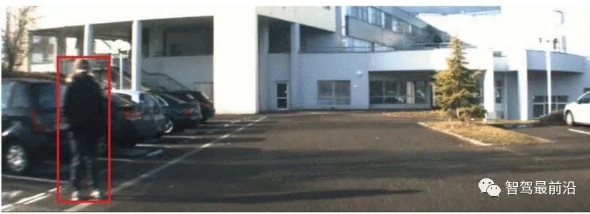
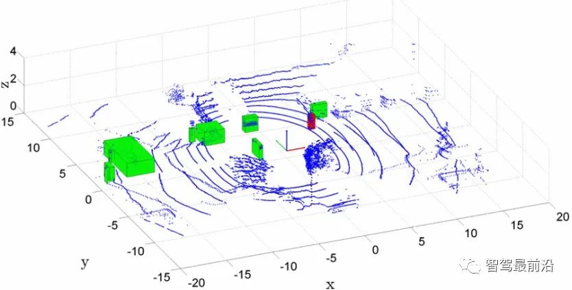
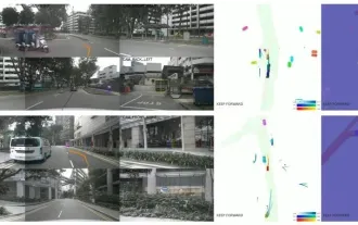
Point clouds were used for the construction of OG according to the method described in Section III based on recorded data sets from four laser scanners. Figure 7 shows the surrounding scene and objects to avoid. The temporal fusion of OG highlights the conflict in describing dynamic units. A hierarchical clustering algorithm (from the Statistics and Machine Learning Toolbox in MATLAB) was applied to construct dynamic objects. They are shown in Figure 8. via 3D bounding box. The displayed coordinates correspond to the vehicle attitude based on GPS data. The objects to avoid are red objects. It can be noted that due to the sensitivity of the method to positioning errors, some erroneous detection results can be found.
 Picture
Figure 7 Sequence for obstacle avoidance test
 Picture
Figure 8 Point cloud, origin coordinates and obstacle detection
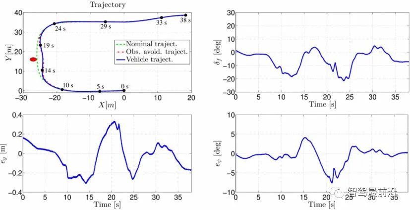
The experimental results are shown in Figure 9. As you can see from the upper left image, the nominal trajectory line intersects the object's position, while the resulting red path avoids obstacles. It can also be observed that the lateral controller ensures good trajectory tracking and avoids detection of obstacles between 13 s and 20 s. During this time interval, the controller generates a steering angle that changes from positive to negative values to avoid obstacles and ensure a small tracking error sum.
 Picture
Figure 9 Steering controller results
7 Conclusion
This paper proposes a dynamic obstacle avoidance scheme based on three levels of perception, path planning and control guidance. Dynamic obstacle detection is performed based on the evidence occupancy grid. Path planning is based on the sigmoïd function to generate smooth trajectories to avoid detecting obstacles. Ultimately, the vehicle follows the vehicle-generated reference trajectory through a lateral control-based strategy at the center of collision. Experimental results on our test vehicle show that this method is effective for obstacle avoidance. Future work will include consideration of positioning strategies and evaluation of this approach in more complex situations.
References
 Pictures
 Image] [image
The above is the detailed content of Detailed explanation of obstacle avoidance, path planning and control technology for autonomous vehicles. For more information, please follow other related articles on the PHP Chinese website!

Hot AI Tools

Undresser.AI Undress
AI-powered app for creating realistic nude photos

AI Clothes Remover
Online AI tool for removing clothes from photos.

Undress AI Tool
Undress images for free

Clothoff.io
AI clothes remover

AI Hentai Generator
Generate AI Hentai for free.

Hot Article
Hot Tools

Notepad++7.3.1
Easy-to-use and free code editor

SublimeText3 Chinese version
Chinese version, very easy to use

Zend Studio 13.0.1
Powerful PHP integrated development environment

Dreamweaver CS6
Visual web development tools

SublimeText3 Mac version
God-level code editing software (SublimeText3)
Hot Topics
 1377
1377
 52
52

 Why is Gaussian Splatting so popular in autonomous driving that NeRF is starting to be abandoned?
Jan 17, 2024 pm 02:57 PM
Why is Gaussian Splatting so popular in autonomous driving that NeRF is starting to be abandoned?
Jan 17, 2024 pm 02:57 PM
Written above & the author’s personal understanding Three-dimensional Gaussiansplatting (3DGS) is a transformative technology that has emerged in the fields of explicit radiation fields and computer graphics in recent years. This innovative method is characterized by the use of millions of 3D Gaussians, which is very different from the neural radiation field (NeRF) method, which mainly uses an implicit coordinate-based model to map spatial coordinates to pixel values. With its explicit scene representation and differentiable rendering algorithms, 3DGS not only guarantees real-time rendering capabilities, but also introduces an unprecedented level of control and scene editing. This positions 3DGS as a potential game-changer for next-generation 3D reconstruction and representation. To this end, we provide a systematic overview of the latest developments and concerns in the field of 3DGS for the first time.
 How to solve the long tail problem in autonomous driving scenarios?
Jun 02, 2024 pm 02:44 PM
How to solve the long tail problem in autonomous driving scenarios?
Jun 02, 2024 pm 02:44 PM
Yesterday during the interview, I was asked whether I had done any long-tail related questions, so I thought I would give a brief summary. The long-tail problem of autonomous driving refers to edge cases in autonomous vehicles, that is, possible scenarios with a low probability of occurrence. The perceived long-tail problem is one of the main reasons currently limiting the operational design domain of single-vehicle intelligent autonomous vehicles. The underlying architecture and most technical issues of autonomous driving have been solved, and the remaining 5% of long-tail problems have gradually become the key to restricting the development of autonomous driving. These problems include a variety of fragmented scenarios, extreme situations, and unpredictable human behavior. The "long tail" of edge scenarios in autonomous driving refers to edge cases in autonomous vehicles (AVs). Edge cases are possible scenarios with a low probability of occurrence. these rare events
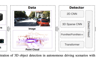 Choose camera or lidar? A recent review on achieving robust 3D object detection
Jan 26, 2024 am 11:18 AM
Choose camera or lidar? A recent review on achieving robust 3D object detection
Jan 26, 2024 am 11:18 AM
0.Written in front&& Personal understanding that autonomous driving systems rely on advanced perception, decision-making and control technologies, by using various sensors (such as cameras, lidar, radar, etc.) to perceive the surrounding environment, and using algorithms and models for real-time analysis and decision-making. This enables vehicles to recognize road signs, detect and track other vehicles, predict pedestrian behavior, etc., thereby safely operating and adapting to complex traffic environments. This technology is currently attracting widespread attention and is considered an important development area in the future of transportation. one. But what makes autonomous driving difficult is figuring out how to make the car understand what's going on around it. This requires that the three-dimensional object detection algorithm in the autonomous driving system can accurately perceive and describe objects in the surrounding environment, including their locations,
 The Stable Diffusion 3 paper is finally released, and the architectural details are revealed. Will it help to reproduce Sora?
Mar 06, 2024 pm 05:34 PM
The Stable Diffusion 3 paper is finally released, and the architectural details are revealed. Will it help to reproduce Sora?
Mar 06, 2024 pm 05:34 PM
StableDiffusion3’s paper is finally here! This model was released two weeks ago and uses the same DiT (DiffusionTransformer) architecture as Sora. It caused quite a stir once it was released. Compared with the previous version, the quality of the images generated by StableDiffusion3 has been significantly improved. It now supports multi-theme prompts, and the text writing effect has also been improved, and garbled characters no longer appear. StabilityAI pointed out that StableDiffusion3 is a series of models with parameter sizes ranging from 800M to 8B. This parameter range means that the model can be run directly on many portable devices, significantly reducing the use of AI
 This article is enough for you to read about autonomous driving and trajectory prediction!
Feb 28, 2024 pm 07:20 PM
This article is enough for you to read about autonomous driving and trajectory prediction!
Feb 28, 2024 pm 07:20 PM
Trajectory prediction plays an important role in autonomous driving. Autonomous driving trajectory prediction refers to predicting the future driving trajectory of the vehicle by analyzing various data during the vehicle's driving process. As the core module of autonomous driving, the quality of trajectory prediction is crucial to downstream planning control. The trajectory prediction task has a rich technology stack and requires familiarity with autonomous driving dynamic/static perception, high-precision maps, lane lines, neural network architecture (CNN&GNN&Transformer) skills, etc. It is very difficult to get started! Many fans hope to get started with trajectory prediction as soon as possible and avoid pitfalls. Today I will take stock of some common problems and introductory learning methods for trajectory prediction! Introductory related knowledge 1. Are the preview papers in order? A: Look at the survey first, p
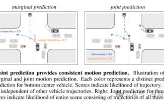
 SIMPL: A simple and efficient multi-agent motion prediction benchmark for autonomous driving
Feb 20, 2024 am 11:48 AM
SIMPL: A simple and efficient multi-agent motion prediction benchmark for autonomous driving
Feb 20, 2024 am 11:48 AM
Original title: SIMPL: ASimpleandEfficientMulti-agentMotionPredictionBaselineforAutonomousDriving Paper link: https://arxiv.org/pdf/2402.02519.pdf Code link: https://github.com/HKUST-Aerial-Robotics/SIMPL Author unit: Hong Kong University of Science and Technology DJI Paper idea: This paper proposes a simple and efficient motion prediction baseline (SIMPL) for autonomous vehicles. Compared with traditional agent-cent
 nuScenes' latest SOTA | SparseAD: Sparse query helps efficient end-to-end autonomous driving!
Apr 17, 2024 pm 06:22 PM
nuScenes' latest SOTA | SparseAD: Sparse query helps efficient end-to-end autonomous driving!
Apr 17, 2024 pm 06:22 PM
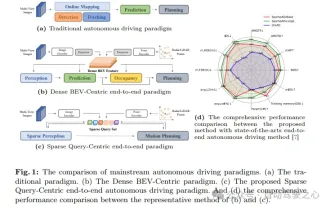
Written in front & starting point The end-to-end paradigm uses a unified framework to achieve multi-tasking in autonomous driving systems. Despite the simplicity and clarity of this paradigm, the performance of end-to-end autonomous driving methods on subtasks still lags far behind single-task methods. At the same time, the dense bird's-eye view (BEV) features widely used in previous end-to-end methods make it difficult to scale to more modalities or tasks. A sparse search-centric end-to-end autonomous driving paradigm (SparseAD) is proposed here, in which sparse search fully represents the entire driving scenario, including space, time, and tasks, without any dense BEV representation. Specifically, a unified sparse architecture is designed for task awareness including detection, tracking, and online mapping. In addition, heavy
 Let's talk about end-to-end and next-generation autonomous driving systems, as well as some misunderstandings about end-to-end autonomous driving?
Apr 15, 2024 pm 04:13 PM
Let's talk about end-to-end and next-generation autonomous driving systems, as well as some misunderstandings about end-to-end autonomous driving?
Apr 15, 2024 pm 04:13 PM
In the past month, due to some well-known reasons, I have had very intensive exchanges with various teachers and classmates in the industry. An inevitable topic in the exchange is naturally end-to-end and the popular Tesla FSDV12. I would like to take this opportunity to sort out some of my thoughts and opinions at this moment for your reference and discussion. How to define an end-to-end autonomous driving system, and what problems should be expected to be solved end-to-end? According to the most traditional definition, an end-to-end system refers to a system that inputs raw information from sensors and directly outputs variables of concern to the task. For example, in image recognition, CNN can be called end-to-end compared to the traditional feature extractor + classifier method. In autonomous driving tasks, input data from various sensors (camera/LiDAR
