

Machine Learning | PyTorch Concise Tutorial Part 2

Following the previous article "PyTorch Concise Tutorial Part 1" , continue to learn multi-layer perceptron, convolutional neural network and LSTMNet.
1. Multi-layer perceptron
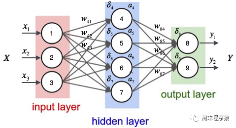
The multi-layer perceptron is a simple neural network and an important foundation for deep learning. It overcomes the limitations of linear models by adding one or more hidden layers to the network. The specific diagram is as follows:
import numpy as npimport torchfrom torch.autograd import Variablefrom torch import optimfrom data_util import load_mnistdef build_model(input_dim, output_dim):return torch.nn.Sequential(torch.nn.Linear(input_dim, 512, bias=False),torch.nn.ReLU(),torch.nn.Dropout(0.2),torch.nn.Linear(512, 512, bias=False),torch.nn.ReLU(),torch.nn.Dropout(0.2),torch.nn.Linear(512, output_dim, bias=False),)def train(model, loss, optimizer, x_val, y_val):model.train()optimizer.zero_grad()fx = model.forward(x_val)output = loss.forward(fx, y_val)output.backward()optimizer.step()return output.item()def predict(model, x_val):model.eval()output = model.forward(x_val)return output.data.numpy().argmax(axis=1)def main():torch.manual_seed(42)trX, teX, trY, teY = load_mnist(notallow=False)trX = torch.from_numpy(trX).float()teX = torch.from_numpy(teX).float()trY = torch.tensor(trY)n_examples, n_features = trX.size()n_classes = 10model = build_model(n_features, n_classes)loss = torch.nn.CrossEntropyLoss(reductinotallow='mean')optimizer = optim.Adam(model.parameters())batch_size = 100for i in range(100):cost = 0.num_batches = n_examples // batch_sizefor k in range(num_batches):start, end = k * batch_size, (k + 1) * batch_sizecost += train(model, loss, optimizer,trX[start:end], trY[start:end])predY = predict(model, teX)print("Epoch %d, cost = %f, acc = %.2f%%"% (i + 1, cost / num_batches, 100. * np.mean(predY == teY)))if __name__ == "__main__":main()(1) The above code is similar to the code of a single-layer neural network. The difference is that build_model builds a layer containing three linear layers and two ReLU Neural network model of activation function:
- Add the first linear layer to the model, the number of input features of this layer is input_dim, and the number of output features is 512;
- Then add a ReLU activation function and a Dropout layer are used to enhance the nonlinear capability of the model and prevent overfitting;
- Add a second linear layer to the model, the number of input features of this layer is 512, and the number of output features is 512;
- Then add a ReLU activation function and a Dropout layer;
- Add a third linear layer to the model, the number of input features of this layer is 512, and the number of output features is output_dim , that is, the number of output categories of the model;
(2) What is the ReLU activation function? The ReLU (Rectified Linear Unit) activation function is a commonly used activation function in deep learning and neural networks. The mathematical expression of the ReLU function is: f(x) = max(0, x), where x is the input value. The characteristic of the ReLU function is that when the input value is less than or equal to 0, the output is 0; when the input value is greater than 0, the output is equal to the input value. Simply put, the ReLU function suppresses the negative part to 0 and leaves the positive part unchanged. The role of the ReLU activation function in the neural network is to introduce nonlinear factors so that the neural network can fit complex nonlinear relationships. At the same time, the ReLU function has fast calculation speed and fast convergence speed compared to other activation functions (such as Sigmoid or Tanh). and other advantages;
(3) What is the Dropout layer? Dropout layer is a technique used in neural networks to prevent overfitting. During the training process, the Dropout layer will randomly set the output of some neurons to 0, that is, "discard" these neurons. The purpose of this is to reduce the interdependence between neurons and thereby improve the generalization ability of the network. ;
(4)print("Epoch %d, cost = %f, acc = %.2f%%" % (i 1, cost / num_batches, 100. * np.mean(predY == teY ))) Finally, print the current training round, loss value and acc. The above code output is as follows:
...Epoch 91, cost = 0.011129, acc = 98.45%Epoch 92, cost = 0.007644, acc = 98.58%Epoch 93, cost = 0.011872, acc = 98.61%Epoch 94, cost = 0.010658, acc = 98.58%Epoch 95, cost = 0.007274, acc = 98.54%Epoch 96, cost = 0.008183, acc = 98.43%Epoch 97, cost = 0.009999, acc = 98.33%Epoch 98, cost = 0.011613, acc = 98.36%Epoch 99, cost = 0.007391, acc = 98.51%Epoch 100, cost = 0.011122, acc = 98.59%
It can be seen that the same data classification in the end has a higher accuracy than the single-layer neural network (98.59% > 97.68%).
2. Convolutional Neural Network
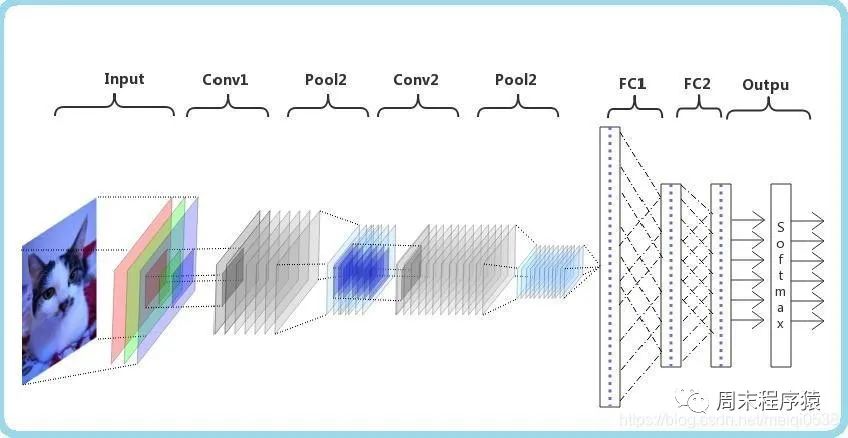
Convolutional neural network (CNN) is a deep learning algorithm. When a matrix is input, CNN can distinguish between important and unimportant parts (assign weights). Compared with other classification tasks, CNN does not require high data preprocessing. As long as it is fully trained, it can learn the characteristics of the matrix. The following figure shows the process:
import numpy as npimport torchfrom torch.autograd import Variablefrom torch import optimfrom data_util import load_mnistclass ConvNet(torch.nn.Module):def __init__(self, output_dim):super(ConvNet, self).__init__()self.conv = torch.nn.Sequential()self.conv.add_module("conv_1", torch.nn.Conv2d(1, 10, kernel_size=5))self.conv.add_module("maxpool_1", torch.nn.MaxPool2d(kernel_size=2))self.conv.add_module("relu_1", torch.nn.ReLU())self.conv.add_module("conv_2", torch.nn.Conv2d(10, 20, kernel_size=5))self.conv.add_module("dropout_2", torch.nn.Dropout())self.conv.add_module("maxpool_2", torch.nn.MaxPool2d(kernel_size=2))self.conv.add_module("relu_2", torch.nn.ReLU())self.fc = torch.nn.Sequential()self.fc.add_module("fc1", torch.nn.Linear(320, 50))self.fc.add_module("relu_3", torch.nn.ReLU())self.fc.add_module("dropout_3", torch.nn.Dropout())self.fc.add_module("fc2", torch.nn.Linear(50, output_dim))def forward(self, x):x = self.conv.forward(x)x = x.view(-1, 320)return self.fc.forward(x)def train(model, loss, optimizer, x_val, y_val):model.train()optimizer.zero_grad()fx = model.forward(x_val)output = loss.forward(fx, y_val)output.backward()optimizer.step()return output.item()def predict(model, x_val):model.eval()output = model.forward(x_val)return output.data.numpy().argmax(axis=1)def main():torch.manual_seed(42)trX, teX, trY, teY = load_mnist(notallow=False)trX = trX.reshape(-1, 1, 28, 28)teX = teX.reshape(-1, 1, 28, 28)trX = torch.from_numpy(trX).float()teX = torch.from_numpy(teX).float()trY = torch.tensor(trY)n_examples = len(trX)n_classes = 10model = ConvNet(output_dim=n_classes)loss = torch.nn.CrossEntropyLoss(reductinotallow='mean')optimizer = optim.SGD(model.parameters(), lr=0.01, momentum=0.9)batch_size = 100for i in range(100):cost = 0.num_batches = n_examples // batch_sizefor k in range(num_batches):start, end = k * batch_size, (k + 1) * batch_sizecost += train(model, loss, optimizer,trX[start:end], trY[start:end])predY = predict(model, teX)print("Epoch %d, cost = %f, acc = %.2f%%"% (i + 1, cost / num_batches, 100. * np.mean(predY == teY)))if __name__ == "__main__":main() (1) The above code defines a class named ConvNet, which inherits from the torch.nn.Module class and represents a volume Convolutional neural network defines two sub-modules conv and fc in the __init__ method, which represent the convolutional layer and the fully connected layer respectively. In the conv submodule, we define two convolutional layers (torch.nn.Conv2d), two maximum pooling layers (torch.nn.MaxPool2d), two ReLU activation functions (torch.nn.ReLU) and a Dropout layer (torch.nn.Dropout). In the fc sub-module, two linear layers (torch.nn.Linear), a ReLU activation function and a Dropout layer are defined;
The pooling layer plays an important role in CNN, Its main purposes are as follows:
- 降低维度:池化层通过对输入特征图(Feature maps)进行局部区域的下采样操作,降低了特征图的尺寸。这样可以减少后续层中的参数数量,降低计算复杂度,加速训练过程;
- 平移不变性:池化层可以提高网络对输入图像的平移不变性。当图像中的某个特征发生小幅度平移时,池化层的输出仍然具有相似的特征表示。这有助于提高模型的泛化能力,使其能够在不同位置和尺度下识别相同的特征;
- 防止过拟合:通过减少特征图的尺寸,池化层可以降低模型的参数数量,从而降低过拟合的风险;
- 增强特征表达:池化操作可以聚合局部区域内的特征,从而强化和突出更重要的特征信息。常见的池化操作有最大池化(Max Pooling)和平均池化(Average Pooling),分别表示在局部区域内取最大值或平均值作为输出;
(3)print("Epoch %d, cost = %f, acc = %.2f%%" % (i + 1, cost / num_batches, 100. * np.mean(predY == teY)))最后打印当前训练的轮次,损失值和acc,上述的代码输出如下:
...Epoch 91, cost = 0.047302, acc = 99.22%Epoch 92, cost = 0.049026, acc = 99.22%Epoch 93, cost = 0.048953, acc = 99.13%Epoch 94, cost = 0.045235, acc = 99.12%Epoch 95, cost = 0.045136, acc = 99.14%Epoch 96, cost = 0.048240, acc = 99.02%Epoch 97, cost = 0.049063, acc = 99.21%Epoch 98, cost = 0.045373, acc = 99.23%Epoch 99, cost = 0.046127, acc = 99.12%Epoch 100, cost = 0.046864, acc = 99.10%
可以看出最后相同的数据分类,准确率比多层感知机要高(99.10% > 98.59%)。
3、LSTMNet
LSTMNet是使用长短时记忆网络(Long Short-Term Memory, LSTM)构建的神经网络,核心思想是引入了一个名为"记忆单元"的结构,该结构可以在一定程度上保留长期依赖信息,LSTM中的每个单元包括一个输入门(input gate)、一个遗忘门(forget gate)和一个输出门(output gate),这些门的作用是控制信息在记忆单元中的流动,以便网络可以学习何时存储、更新或输出有用的信息。
import numpy as npimport torchfrom torch import optim, nnfrom data_util import load_mnistclass LSTMNet(torch.nn.Module):def __init__(self, input_dim, hidden_dim, output_dim):super(LSTMNet, self).__init__()self.hidden_dim = hidden_dimself.lstm = nn.LSTM(input_dim, hidden_dim)self.linear = nn.Linear(hidden_dim, output_dim, bias=False)def forward(self, x):batch_size = x.size()[1]h0 = torch.zeros([1, batch_size, self.hidden_dim])c0 = torch.zeros([1, batch_size, self.hidden_dim])fx, _ = self.lstm.forward(x, (h0, c0))return self.linear.forward(fx[-1])def train(model, loss, optimizer, x_val, y_val):model.train()optimizer.zero_grad()fx = model.forward(x_val)output = loss.forward(fx, y_val)output.backward()optimizer.step()return output.item()def predict(model, x_val):model.eval()output = model.forward(x_val)return output.data.numpy().argmax(axis=1)def main():torch.manual_seed(42)trX, teX, trY, teY = load_mnist(notallow=False)train_size = len(trY)n_classes = 10seq_length = 28input_dim = 28hidden_dim = 128batch_size = 100epochs = 100trX = trX.reshape(-1, seq_length, input_dim)teX = teX.reshape(-1, seq_length, input_dim)trX = np.swapaxes(trX, 0, 1)teX = np.swapaxes(teX, 0, 1)trX = torch.from_numpy(trX).float()teX = torch.from_numpy(teX).float()trY = torch.tensor(trY)model = LSTMNet(input_dim, hidden_dim, n_classes)loss = torch.nn.CrossEntropyLoss(reductinotallow='mean')optimizer = optim.SGD(model.parameters(), lr=0.01, momentum=0.9)for i in range(epochs):cost = 0.num_batches = train_size // batch_sizefor k in range(num_batches):start, end = k * batch_size, (k + 1) * batch_sizecost += train(model, loss, optimizer,trX[:, start:end, :], trY[start:end])predY = predict(model, teX)print("Epoch %d, cost = %f, acc = %.2f%%" %(i + 1, cost / num_batches, 100. * np.mean(predY == teY)))if __name__ == "__main__":main()(1)以上这段代码通用的部分就不解释了,具体说LSTMNet类:
- self.lstm = nn.LSTM(input_dim, hidden_dim)创建一个LSTM层,输入维度为input_dim,隐藏层维度为hidden_dim;
- self.linear = nn.Linear(hidden_dim, output_dim, bias=False)创建一个线性层(全连接层),输入维度为hidden_dim,输出维度为output_dim,并设置不使用偏置项(bias);
- h0 = torch.zeros([1, batch_size, self.hidden_dim])初始化LSTM层的隐藏状态h0,全零张量,形状为[1, batch_size, hidden_dim];
- c0 = torch.zeros([1, batch_size, self.hidden_dim])初始化LSTM层的细胞状态c0,全零张量,形状为[1, batch_size, hidden_dim];
- fx, _ = self.lstm.forward(x, (h0, c0))将输入数据x以及初始隐藏状态h0和细胞状态c0传入LSTM层,得到LSTM层的输出fx;
- return self.linear.forward(fx[-1])将LSTM层的输出传入线性层进行计算,得到最终输出。这里fx[-1]表示取LSTM层输出的最后一个时间步的数据;
(2)print("第%d轮,损失值=%f,准确率=%.2f%%" % (i + 1, cost / num_batches, 100. * np.mean(predY == teY)))。打印出当前训练轮次的信息,其中包括损失值和准确率,以上代码的输出结果如下:
Epoch 91, cost = 0.000468, acc = 98.57%Epoch 92, cost = 0.000452, acc = 98.57%Epoch 93, cost = 0.000437, acc = 98.58%Epoch 94, cost = 0.000422, acc = 98.57%Epoch 95, cost = 0.000409, acc = 98.58%Epoch 96, cost = 0.000396, acc = 98.58%Epoch 97, cost = 0.000384, acc = 98.57%Epoch 98, cost = 0.000372, acc = 98.56%Epoch 99, cost = 0.000360, acc = 98.55%Epoch 100, cost = 0.000349, acc = 98.55%
4、辅助代码
两篇文章的from data_util import load_mnist的data_util.py代码如下:
import gzip
import os
import urllib.request as request
from os import path
import numpy as np

DATASET_DIR = 'datasets/'
MNIST_FILES = ["train-images-idx3-ubyte.gz", "train-labels-idx1-ubyte.gz", "t10k-images-idx3-ubyte.gz", "t10k-labels-idx1-ubyte.gz"]

def download_file(url, local_path):
    dir_path = path.dirname(local_path)
    if not path.exists(dir_path):
        print("创建目录'%s' ..." % dir_path)
        os.makedirs(dir_path)
    print("从'%s'下载中 ..." % url)
    request.urlretrieve(url, local_path)

def download_mnist(local_path):
    url_root = "http://yann.lecun.com/exdb/mnist/"
    for f_name in MNIST_FILES:
        f_path = os.path.join(local_path, f_name)
        if not path.exists(f_path):
            download_file(url_root + f_name, f_path)

def one_hot(x, n):
    if type(x) == list:
        x = np.array(x)
    x = x.flatten()
    o_h = np.zeros((len(x), n))
    o_h[np.arange(len(x)), x] = 1
    return o_h

def load_mnist(ntrain=60000, ntest=10000, notallow=True):
    data_dir = os.path.join(DATASET_DIR, 'mnist/')
    if not path.exists(data_dir):
        download_mnist(data_dir)
    else:
        # 检查所有文件
        checks = [path.exists(os.path.join(data_dir, f)) for f in MNIST_FILES]
        if not np.all(checks):
            download_mnist(data_dir)

    with gzip.open(os.path.join(data_dir, 'train-images-idx3-ubyte.gz')) as fd:
        buf = fd.read()
        loaded = np.frombuffer(buf, dtype=np.uint8)
        trX = loaded[16:].reshape((60000, 28 * 28)).astype(float)

    with gzip.open(os.path.join(data_dir, 'train-labels-idx1-ubyte.gz')) as fd:
        buf = fd.read()
        loaded = np.frombuffer(buf, dtype=np.uint8)
        trY = loaded[8:].reshape((60000))

    with gzip.open(os.path.join(data_dir, 't10k-images-idx3-ubyte.gz')) as fd:
        buf = fd.read()
        loaded = np.frombuffer(buf, dtype=np.uint8)
        teX = loaded[16:].reshape((10000, 28 * 28)).astype(float)

    with gzip.open(os.path.join(data_dir, 't10k-labels-idx1-ubyte.gz')) as fd:
        buf = fd.read()
        loaded = np.frombuffer(buf, dtype=np.uint8)
        teY = loaded[8:].reshape((10000))

    trX /= 255.
    teX /= 255.
    trX = trX[:ntrain]
    trY = trY[:ntrain]
    teX = teX[:ntest]
    teY = teY[:ntest]

    if onehot:
        trY = one_hot(trY, 10)
        teY = one_hot(teY, 10)
    else:
        trY = np.asarray(trY)
        teY = np.asarray(teY)

return trX, teX, trY, teYThe above is the detailed content of Machine Learning | PyTorch Concise Tutorial Part 2. For more information, please follow other related articles on the PHP Chinese website!

Hot AI Tools

Undresser.AI Undress
AI-powered app for creating realistic nude photos

AI Clothes Remover
Online AI tool for removing clothes from photos.

Undress AI Tool
Undress images for free

Clothoff.io
AI clothes remover

AI Hentai Generator
Generate AI Hentai for free.

Hot Article
Hot Tools

Notepad++7.3.1
Easy-to-use and free code editor

SublimeText3 Chinese version
Chinese version, very easy to use

Zend Studio 13.0.1
Powerful PHP integrated development environment

Dreamweaver CS6
Visual web development tools

SublimeText3 Mac version
God-level code editing software (SublimeText3)
Hot Topics
 1377
1377
 52
52

 15 recommended open source free image annotation tools
Mar 28, 2024 pm 01:21 PM
15 recommended open source free image annotation tools
Mar 28, 2024 pm 01:21 PM
Image annotation is the process of associating labels or descriptive information with images to give deeper meaning and explanation to the image content. This process is critical to machine learning, which helps train vision models to more accurately identify individual elements in images. By adding annotations to images, the computer can understand the semantics and context behind the images, thereby improving the ability to understand and analyze the image content. Image annotation has a wide range of applications, covering many fields, such as computer vision, natural language processing, and graph vision models. It has a wide range of applications, such as assisting vehicles in identifying obstacles on the road, and helping in the detection and diagnosis of diseases through medical image recognition. . This article mainly recommends some better open source and free image annotation tools. 1.Makesens
 This article will take you to understand SHAP: model explanation for machine learning
Jun 01, 2024 am 10:58 AM
This article will take you to understand SHAP: model explanation for machine learning
Jun 01, 2024 am 10:58 AM
In the fields of machine learning and data science, model interpretability has always been a focus of researchers and practitioners. With the widespread application of complex models such as deep learning and ensemble methods, understanding the model's decision-making process has become particularly important. Explainable AI|XAI helps build trust and confidence in machine learning models by increasing the transparency of the model. Improving model transparency can be achieved through methods such as the widespread use of multiple complex models, as well as the decision-making processes used to explain the models. These methods include feature importance analysis, model prediction interval estimation, local interpretability algorithms, etc. Feature importance analysis can explain the decision-making process of a model by evaluating the degree of influence of the model on the input features. Model prediction interval estimate
 Transparent! An in-depth analysis of the principles of major machine learning models!
Apr 12, 2024 pm 05:55 PM
Transparent! An in-depth analysis of the principles of major machine learning models!
Apr 12, 2024 pm 05:55 PM
In layman’s terms, a machine learning model is a mathematical function that maps input data to a predicted output. More specifically, a machine learning model is a mathematical function that adjusts model parameters by learning from training data to minimize the error between the predicted output and the true label. There are many models in machine learning, such as logistic regression models, decision tree models, support vector machine models, etc. Each model has its applicable data types and problem types. At the same time, there are many commonalities between different models, or there is a hidden path for model evolution. Taking the connectionist perceptron as an example, by increasing the number of hidden layers of the perceptron, we can transform it into a deep neural network. If a kernel function is added to the perceptron, it can be converted into an SVM. this one
 Identify overfitting and underfitting through learning curves
Apr 29, 2024 pm 06:50 PM
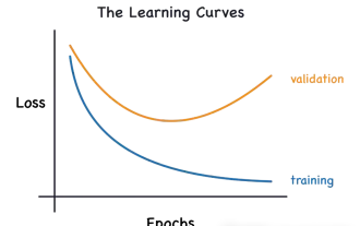
Identify overfitting and underfitting through learning curves
Apr 29, 2024 pm 06:50 PM
This article will introduce how to effectively identify overfitting and underfitting in machine learning models through learning curves. Underfitting and overfitting 1. Overfitting If a model is overtrained on the data so that it learns noise from it, then the model is said to be overfitting. An overfitted model learns every example so perfectly that it will misclassify an unseen/new example. For an overfitted model, we will get a perfect/near-perfect training set score and a terrible validation set/test score. Slightly modified: "Cause of overfitting: Use a complex model to solve a simple problem and extract noise from the data. Because a small data set as a training set may not represent the correct representation of all data." 2. Underfitting Heru
 The evolution of artificial intelligence in space exploration and human settlement engineering
Apr 29, 2024 pm 03:25 PM
The evolution of artificial intelligence in space exploration and human settlement engineering
Apr 29, 2024 pm 03:25 PM
In the 1950s, artificial intelligence (AI) was born. That's when researchers discovered that machines could perform human-like tasks, such as thinking. Later, in the 1960s, the U.S. Department of Defense funded artificial intelligence and established laboratories for further development. Researchers are finding applications for artificial intelligence in many areas, such as space exploration and survival in extreme environments. Space exploration is the study of the universe, which covers the entire universe beyond the earth. Space is classified as an extreme environment because its conditions are different from those on Earth. To survive in space, many factors must be considered and precautions must be taken. Scientists and researchers believe that exploring space and understanding the current state of everything can help understand how the universe works and prepare for potential environmental crises
 Implementing Machine Learning Algorithms in C++: Common Challenges and Solutions
Jun 03, 2024 pm 01:25 PM
Implementing Machine Learning Algorithms in C++: Common Challenges and Solutions
Jun 03, 2024 pm 01:25 PM
Common challenges faced by machine learning algorithms in C++ include memory management, multi-threading, performance optimization, and maintainability. Solutions include using smart pointers, modern threading libraries, SIMD instructions and third-party libraries, as well as following coding style guidelines and using automation tools. Practical cases show how to use the Eigen library to implement linear regression algorithms, effectively manage memory and use high-performance matrix operations.
 Explainable AI: Explaining complex AI/ML models
Jun 03, 2024 pm 10:08 PM
Explainable AI: Explaining complex AI/ML models
Jun 03, 2024 pm 10:08 PM
Translator | Reviewed by Li Rui | Chonglou Artificial intelligence (AI) and machine learning (ML) models are becoming increasingly complex today, and the output produced by these models is a black box – unable to be explained to stakeholders. Explainable AI (XAI) aims to solve this problem by enabling stakeholders to understand how these models work, ensuring they understand how these models actually make decisions, and ensuring transparency in AI systems, Trust and accountability to address this issue. This article explores various explainable artificial intelligence (XAI) techniques to illustrate their underlying principles. Several reasons why explainable AI is crucial Trust and transparency: For AI systems to be widely accepted and trusted, users need to understand how decisions are made
 Five schools of machine learning you don't know about
Jun 05, 2024 pm 08:51 PM
Five schools of machine learning you don't know about
Jun 05, 2024 pm 08:51 PM
Machine learning is an important branch of artificial intelligence that gives computers the ability to learn from data and improve their capabilities without being explicitly programmed. Machine learning has a wide range of applications in various fields, from image recognition and natural language processing to recommendation systems and fraud detection, and it is changing the way we live. There are many different methods and theories in the field of machine learning, among which the five most influential methods are called the "Five Schools of Machine Learning". The five major schools are the symbolic school, the connectionist school, the evolutionary school, the Bayesian school and the analogy school. 1. Symbolism, also known as symbolism, emphasizes the use of symbols for logical reasoning and expression of knowledge. This school of thought believes that learning is a process of reverse deduction, through existing
