

Commonly used algorithms in timing analysis are all here

Time series analysis is to use the characteristics of an event in the past period to predict the characteristics of the event in the future period. This is a relatively complex predictive modeling problem that is different from the predictions of regression analysis models. The time series model depends on the order in which events occur. Values of the same size will produce different results if the order is changed.

See all timing issues It is a regression problem, but there are certain differences in the regression methods (linear regression, tree model, deep learning, etc.).
Timing analysis includes static timing analysis (STA) and dynamic timing analysis.
The following are several common timing analysis algorithms
1 Deep learning timing analysis
RNN (Recurrent Neural Network)
Recurrent neural network refers to a structure that occurs repeatedly over time. It has a very wide range of applications in natural language processing (NLP), speech images and other fields. The biggest difference between RNN networks and other networks is that RNN can achieve a certain "memory function" and is the best choice for time series analysis. Just like human beings can better understand the world through their own past memories. RNN also implements a mechanism similar to that of the human brain, retaining a certain amount of memory for the processed information, unlike other types of neural networks that cannot retain memory for the processed information.
Advantages:
This method can memorize time and is suitable for solving problems with short intervals in the time series
Disadvantages:
Long-term step data is prone to gradient disappearance and gradient explosion problems
LSTM (Long Short-Term Memory Network)
LSTM (Long Short-Term Memory Network) Memory Network (Long Short-Term Memory) is a temporal recurrent neural network designed to solve the long-term dependency problem existing in conventional recurrent neural networks (RNN). All RNNs are composed of a series of repeated neural network modules
Strengths:
Suitable for processing and predicting important events with very long intervals and delays in time series.
Disadvantages:
Too many model parameters will lead to overfitting problems
2 Traditional time series analysis model
- Auto Regression (AR)
- Moving Average (MA)
- Autoregressive Moving Average (ARMA)
- Autoregressive Integrated Moving Average (ARIMA)
- Seasonal Autoregressive Integrated Moving Average (SARIMA)
- Seasonal Autoregressive Integrated Moving Average with exogenous regressor (Seasonal Autoregressive Integrated Moving-Average with Exogenous Regressors, SARIMAX)
Autoregressive Model AR
Autoregressive Model (AR model for short) is a time series analysis method. Used to describe the relationship between a time series variable and its past values. The AR model assumes a linear relationship between current observations and past observations, and uses past observations to predict future observations.
Strengths:
- Simplicity: The AR model is a linear model that is easy to understand and implement. It only uses past observations as independent variables, with no other complex factors to consider.
- Modeling capabilities: AR models can capture the autocorrelation structure of time series data, that is, the relationship between current observations and past observations. It provides predictions of future observations and reveals trends and patterns in the data.
shortcoming:
- Only applicable to stationary series: The AR model requires that the time series is stationary, that is, the mean, variance and autocorrelation do not change with time. If the series is non-stationary, you may need to perform differentiating operations or use other models to handle the non-stationarity.
- Sensitive to past observations: The prediction results of the AR model are affected by past observations, so the problem of error accumulation may occur when dealing with long-term predictions. A larger order may lead to model overfitting, while a smaller order may not capture the complex dynamics of the time series.
- Unable to handle seasonal data: The AR model cannot directly handle time series with obvious seasonality. For data with seasonal patterns, seasonal AR models (SAR) or ARIMA models can be used for modeling.
Moving Average Method (MA)
Moving Average Method (MA): This method is based on the average of the data and assumes that future values are consistent with There is a certain stability between past values
Strengths:
Be able to capture the moving average relationship in time series data. The MA model utilizes a linear combination of white noise error terms from past time steps to predict current observations and therefore captures the moving average nature in the data.
Relatively simple and intuitive. The parameters of the MA model represent the weights of the white noise error terms at past time steps, and the model can be fitted by estimating these weights.
Disadvantages:
- can only capture the moving average relationship, but cannot capture the autoregressive relationship. The MA model ignores past time step observations and may not capture autocorrelation in the data.
- For some time series data, the MA model may require a higher order to fit the data well, resulting in increased model complexity.
Autoregressive Moving Average Model
Autoregressive Moving Average Model (ARMA model, Auto-Regression and Moving AverageModel) is an important method for studying time series. It is "mixed" based on the autoregressive model (AR model) and the moving average model (MA model). It has the characteristics of wide application range and small prediction error.
Autoregressive Integrated Moving Average (ARIMA)
The ARIMA model is the abbreviation of the autoregressive difference moving average model, and the full name is Autoregressive Integrated Moving Average Model. This model mainly consists of three parts, namely the autoregressive model (AR), the difference process (I) and the moving average model (MA)
The basic idea of the ARIMA model is to use data Use its own historical information to predict the future. The tag value at a point in time is affected by both the tag value in the past period and accidental events in the past period. In other words, the ARIMA model assumes that the tag value fluctuates around the general trend of time. , where the trend is affected by historical labels, fluctuations are affected by accidental events within a period of time, and the general trend itself is not necessarily stable
ARIMA model is a The time series analysis method extracts the time series patterns hidden in the data by modeling the autocorrelation and difference of the data, and then predicts the future data
- AR part Used to process the autoregressive part of a time series, which takes into account the impact of observations from past periods on the current value.
- Part I is used to make the non-stationary time series stationary. Through first-order or second-order difference processing, the trend and seasonal factors in the time series are eliminated.
- The MA part is used to process the moving average part of the time series, which takes into account the impact of past prediction errors on the current value.
Combining these three parts, the ARIMA model can not only capture the trend changes of the data, but also handle data with temporary, sudden changes or large noise. Therefore, the ARIMA model performs well in many time series forecasting problems.
Strengths:
The construction of the model is very simple, only using endogenous variables without resorting to other exogenous variables. The so-called endogenous variables refer to variables that only depend on the data itself, unlike regression models that require the support of other variables
Disadvantages:
The requirement for time series data is stability , or become stable after differential processing
In essence, it can only capture linear relationships, but not non-linear relationships.
Seasonal Autoregressive Integrated Moving Average Model SARIMA
SARIMA is a commonly used time series analysis method, which is an extension of the ARIMA model on seasonal data. SARIMA models can be used to predict seasonal time series data, such as annual sales or weekly website visits. The following are the advantages and disadvantages of the SARIMA model:
Strengths:
- The SARIMA model can handle seasonal data well because it takes into account the time series data seasonal factors.
- The SARIMA model can make long-term forecasts on time series data because it can capture trends and cyclical changes in the data.
- The SARIMA model can be used for multi-variable time series data because it can consider the relationship between multiple variables at the same time.
Disadvantages:
- The SARIMA model requires a large amount of historical data to train, so it may not be suitable when the amount of data is small.
- The SARIMA model is sensitive to outliers, so outliers need to be processed.
- The SARIMA model has a high computational complexity and requires a lot of calculations and optimization.
Seasonal Autoregressive Integrated Moving Average Model SARIMAX with Exogenous Regressor
Seasonal Autoregressive Integrated Moving Average Model (SARIMAX) is a model in the difference A model based on the moving autoregressive model (ARIMA) plus exogenous regressors. It is suitable for time series data with obvious periodic and seasonal characteristics
3 Other time series models
This type of method is represented by lightgbm and xgboost. Generally, Time series problems are converted into supervised learning and predicted through feature engineering and machine learning methods; this model can solve the vast majority of complex time series prediction models. Supports complex data modeling, multi-variable collaborative regression, and nonlinear problems.
The importance of feature engineering is self-evident, and it plays a key role in the success of machine learning. However, feature engineering is not a simple task and requires complex manual processing and unique expertise. The level of feature engineering often determines the upper limit of machine learning, and the machine learning algorithm is just as close to this upper limit as possible. Once the feature engineering is completed, we can directly apply the tree model algorithms - lightgbm and xgboost. These two models are very common and efficient modeling methods. In addition, they also have the following characteristics:
- Fast calculation speed and high model accuracy;
- Missing values are not required Processing is more convenient;
- supports category variables;
- supports feature crossover.
#The specific method to choose needs to be comprehensively considered based on the nature of the data, the characteristics of the problem, and your own experience and abilities.
You need to choose an appropriate time series forecasting method based on specific data characteristics, problem requirements and your own capabilities. Sometimes, combining multiple methods can improve the accuracy and stability of predictions. At the same time, in order to better select models and evaluate prediction results, it is also important to perform visual analysis of data and model diagnosis.
The above is the detailed content of Commonly used algorithms in timing analysis are all here. For more information, please follow other related articles on the PHP Chinese website!

Hot AI Tools

Undresser.AI Undress
AI-powered app for creating realistic nude photos

AI Clothes Remover
Online AI tool for removing clothes from photos.

Undress AI Tool
Undress images for free

Clothoff.io
AI clothes remover

AI Hentai Generator
Generate AI Hentai for free.

Hot Article
Hot Tools

Notepad++7.3.1
Easy-to-use and free code editor

SublimeText3 Chinese version
Chinese version, very easy to use

Zend Studio 13.0.1
Powerful PHP integrated development environment

Dreamweaver CS6
Visual web development tools

SublimeText3 Mac version
God-level code editing software (SublimeText3)
Hot Topics
 1386
1386
 52
52

 Methods and steps for using BERT for sentiment analysis in Python
Jan 22, 2024 pm 04:24 PM
Methods and steps for using BERT for sentiment analysis in Python
Jan 22, 2024 pm 04:24 PM
BERT is a pre-trained deep learning language model proposed by Google in 2018. The full name is BidirectionalEncoderRepresentationsfromTransformers, which is based on the Transformer architecture and has the characteristics of bidirectional encoding. Compared with traditional one-way coding models, BERT can consider contextual information at the same time when processing text, so it performs well in natural language processing tasks. Its bidirectionality enables BERT to better understand the semantic relationships in sentences, thereby improving the expressive ability of the model. Through pre-training and fine-tuning methods, BERT can be used for various natural language processing tasks, such as sentiment analysis, naming
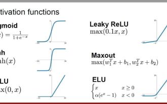 Analysis of commonly used AI activation functions: deep learning practice of Sigmoid, Tanh, ReLU and Softmax
Dec 28, 2023 pm 11:35 PM
Analysis of commonly used AI activation functions: deep learning practice of Sigmoid, Tanh, ReLU and Softmax
Dec 28, 2023 pm 11:35 PM
Activation functions play a crucial role in deep learning. They can introduce nonlinear characteristics into neural networks, allowing the network to better learn and simulate complex input-output relationships. The correct selection and use of activation functions has an important impact on the performance and training results of neural networks. This article will introduce four commonly used activation functions: Sigmoid, Tanh, ReLU and Softmax, starting from the introduction, usage scenarios, advantages, disadvantages and optimization solutions. Dimensions are discussed to provide you with a comprehensive understanding of activation functions. 1. Sigmoid function Introduction to SIgmoid function formula: The Sigmoid function is a commonly used nonlinear function that can map any real number to between 0 and 1. It is usually used to unify the
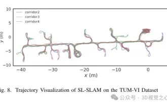 Beyond ORB-SLAM3! SL-SLAM: Low light, severe jitter and weak texture scenes are all handled
May 30, 2024 am 09:35 AM
Beyond ORB-SLAM3! SL-SLAM: Low light, severe jitter and weak texture scenes are all handled
May 30, 2024 am 09:35 AM
Written previously, today we discuss how deep learning technology can improve the performance of vision-based SLAM (simultaneous localization and mapping) in complex environments. By combining deep feature extraction and depth matching methods, here we introduce a versatile hybrid visual SLAM system designed to improve adaptation in challenging scenarios such as low-light conditions, dynamic lighting, weakly textured areas, and severe jitter. sex. Our system supports multiple modes, including extended monocular, stereo, monocular-inertial, and stereo-inertial configurations. In addition, it also analyzes how to combine visual SLAM with deep learning methods to inspire other research. Through extensive experiments on public datasets and self-sampled data, we demonstrate the superiority of SL-SLAM in terms of positioning accuracy and tracking robustness.
 Latent space embedding: explanation and demonstration
Jan 22, 2024 pm 05:30 PM
Latent space embedding: explanation and demonstration
Jan 22, 2024 pm 05:30 PM
Latent Space Embedding (LatentSpaceEmbedding) is the process of mapping high-dimensional data to low-dimensional space. In the field of machine learning and deep learning, latent space embedding is usually a neural network model that maps high-dimensional input data into a set of low-dimensional vector representations. This set of vectors is often called "latent vectors" or "latent encodings". The purpose of latent space embedding is to capture important features in the data and represent them into a more concise and understandable form. Through latent space embedding, we can perform operations such as visualizing, classifying, and clustering data in low-dimensional space to better understand and utilize the data. Latent space embedding has wide applications in many fields, such as image generation, feature extraction, dimensionality reduction, etc. Latent space embedding is the main
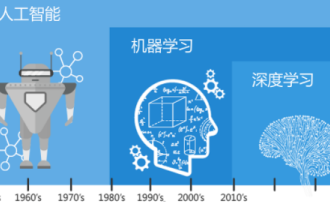 Understand in one article: the connections and differences between AI, machine learning and deep learning
Mar 02, 2024 am 11:19 AM
Understand in one article: the connections and differences between AI, machine learning and deep learning
Mar 02, 2024 am 11:19 AM
In today's wave of rapid technological changes, Artificial Intelligence (AI), Machine Learning (ML) and Deep Learning (DL) are like bright stars, leading the new wave of information technology. These three words frequently appear in various cutting-edge discussions and practical applications, but for many explorers who are new to this field, their specific meanings and their internal connections may still be shrouded in mystery. So let's take a look at this picture first. It can be seen that there is a close correlation and progressive relationship between deep learning, machine learning and artificial intelligence. Deep learning is a specific field of machine learning, and machine learning
 From basics to practice, review the development history of Elasticsearch vector retrieval
Oct 23, 2023 pm 05:17 PM
From basics to practice, review the development history of Elasticsearch vector retrieval
Oct 23, 2023 pm 05:17 PM
1. Introduction Vector retrieval has become a core component of modern search and recommendation systems. It enables efficient query matching and recommendations by converting complex objects (such as text, images, or sounds) into numerical vectors and performing similarity searches in multidimensional spaces. From basics to practice, review the development history of Elasticsearch vector retrieval_elasticsearch As a popular open source search engine, Elasticsearch's development in vector retrieval has always attracted much attention. This article will review the development history of Elasticsearch vector retrieval, focusing on the characteristics and progress of each stage. Taking history as a guide, it is convenient for everyone to establish a full range of Elasticsearch vector retrieval.
 Super strong! Top 10 deep learning algorithms!
Mar 15, 2024 pm 03:46 PM
Super strong! Top 10 deep learning algorithms!
Mar 15, 2024 pm 03:46 PM
Almost 20 years have passed since the concept of deep learning was proposed in 2006. Deep learning, as a revolution in the field of artificial intelligence, has spawned many influential algorithms. So, what do you think are the top 10 algorithms for deep learning? The following are the top algorithms for deep learning in my opinion. They all occupy an important position in terms of innovation, application value and influence. 1. Deep neural network (DNN) background: Deep neural network (DNN), also called multi-layer perceptron, is the most common deep learning algorithm. When it was first invented, it was questioned due to the computing power bottleneck. Until recent years, computing power, The breakthrough came with the explosion of data. DNN is a neural network model that contains multiple hidden layers. In this model, each layer passes input to the next layer and
 AlphaFold 3 is launched, comprehensively predicting the interactions and structures of proteins and all living molecules, with far greater accuracy than ever before
Jul 16, 2024 am 12:08 AM
AlphaFold 3 is launched, comprehensively predicting the interactions and structures of proteins and all living molecules, with far greater accuracy than ever before
Jul 16, 2024 am 12:08 AM
Editor | Radish Skin Since the release of the powerful AlphaFold2 in 2021, scientists have been using protein structure prediction models to map various protein structures within cells, discover drugs, and draw a "cosmic map" of every known protein interaction. . Just now, Google DeepMind released the AlphaFold3 model, which can perform joint structure predictions for complexes including proteins, nucleic acids, small molecules, ions and modified residues. The accuracy of AlphaFold3 has been significantly improved compared to many dedicated tools in the past (protein-ligand interaction, protein-nucleic acid interaction, antibody-antigen prediction). This shows that within a single unified deep learning framework, it is possible to achieve
