Preferred Neural Networks for Application to Time Series Data
| Introduction | This article briefly introduces the development process of recurrent neural network RNN, and analyzes the gradient descent algorithm, backpropagation and LSTM process. |
With the development of science and technology and the substantial improvement of hardware computing capabilities, artificial intelligence has suddenly jumped into people's eyes from decades of behind-the-scenes work. The backbone of artificial intelligence comes from the support of big data, high-performance hardware and excellent algorithms. In 2016, deep learning has become a hot word in Google searches. With AlphaGo defeating the world champion in the Go human-machine battle in the past year or two, people feel that they can no longer resist the rapid advancement of AI. In 2017, AI has made breakthroughs, and related products have also appeared in people's lives, such as intelligent robots, driverless cars, and voice search. Recently, the World Intelligence Conference was successfully held in Tianjin. At the conference, many industry experts and entrepreneurs expressed their views on the future. It can be understood that most technology companies and research institutions are very optimistic about the prospects of artificial intelligence. For example, Baidu will All his wealth is on artificial intelligence, no matter whether he becomes famous or fails after all, as long as he doesn't gain nothing. Why does deep learning suddenly have such a big effect and craze? This is because technology changes life, and many professions may be slowly replaced by artificial intelligence in the future. The whole people are talking about artificial intelligence and deep learning, and even Yann LeCun feels the popularity of artificial intelligence in China!

Closer to home, behind artificial intelligence is big data, excellent algorithms and hardware support with powerful computing capabilities. For example, NVIDIA ranks first among the fifty smartest companies in the world with its strong hardware research and development capabilities and support for deep learning frameworks. In addition, there are many excellent deep learning algorithms, and a new algorithm will appear from time to time, which is really dazzling. But most of them are improved based on classic algorithms, such as convolutional neural network (CNN), deep belief network (DBN), recurrent neural network (RNN), etc.
This article will introduce the classic network Recurrent Neural Network (RNN), which is also the preferred network for time series data. When it comes to certain sequential machine learning tasks, RNN can achieve very high accuracy that no other algorithm can compete with. This is because traditional neural networks only have a short-term memory, while RNN has the advantage of limited short-term memory. However, the first-generation RNNs network did not attract much attention. This is because researchers suffered from serious gradient disappearance problems when using backpropagation and gradient descent algorithms, which hindered the development of RNNs for decades. Finally, a major breakthrough occurred in the late 1990s, leading to a new generation of more accurate RNNs. Nearly two decades after building on that breakthrough, developers perfected and optimized a new generation of RNNs, until apps like Google Voice Search and Apple Siri began to usurp its key processes. Today, RNN networks are spread across every field of research and are helping to ignite a renaissance in artificial intelligence.
Past-Related Neural Networks (RNN)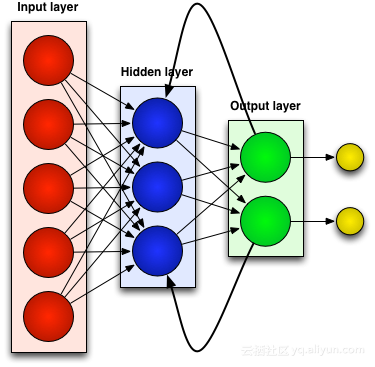
Most artificial neural networks, such as feedforward neural networks, do not remember the input they just received. For example, if a feedforward neural network is fed the character "WISDOM", by the time it reaches the character "D" it has forgotten that it just read the character "S", which is a big problem. No matter how painstakingly the network was trained, it was always difficult to guess the next most likely character "O". This makes it a fairly useless candidate for certain tasks, such as speech recognition, where the quality of recognition largely benefits from the ability to predict the next character. RNN networks, on the other hand, do remember previous inputs, but at a very sophisticated level.
We enter "WISDOM" again and apply it to a recurrent network. The unit or artificial neuron in the RNN network when it receives "D" also has as its input the character "S" it received previously. In other words, it uses the past events combined with the present events as input to predict what will happen next, which gives it the advantage of limited short-term memory. When training, given enough context, it can be guessed that the next character is most likely to be "O".
Adjustment and readjustmentLike all artificial neural networks, RNN units assign a weight matrix to their multiple inputs. These weights represent the proportion of each input in the network layer; a function is then applied to these weights to determine a single output. This The function is generally called a loss function (cost function) and limits the error between the actual output and the target output. However, RNNs not only assign weights to current inputs, but also to inputs from past moments. Then, the weights assigned to the current input and past inputs are dynamically adjusted by minimizing the loss function. This process involves two key concepts: gradient descent and backpropagation (BPTT).
Gradient DescentOne of the most famous algorithms in machine learning is the gradient descent algorithm. Its main advantage is that it significantly avoids the "curse of dimensionality". What is the "curse of dimensionality"? It means that in calculation problems involving vectors, as the number of dimensions increases, the amount of calculation will increase exponentially. This problem plagues many neural network systems because too many variables need to be calculated to achieve the minimum loss function. However, the gradient descent algorithm breaks the curse of dimensionality by amplifying multidimensional errors or local minima of the cost function. This helps the system adjust the weight values assigned to individual units to make the network more precise.
Backpropagation through timeRNN trains its units by fine-tuning its weights through backward inference. Simply put, based on the error between the total output calculated by the unit and the target output, reverse layer-by-layer regression is performed from the final output end of the network, and the partial derivative of the loss function is used to adjust the weight of each unit. This is the famous BP algorithm. For information about the BP algorithm, you can read this blogger’s previous related blogs. The RNN network uses a similar version called backpropagation through time (BPTT). This version extends the tuning process to include weights responsible for the memory of each unit corresponding to the input value at the previous time (T-1).
Yikes: vanishing gradient problem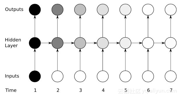
Despite enjoying some initial success with the help of gradient descent algorithms and BPTT, many artificial neural networks (including the first generation RNNs networks) eventually suffered from a serious setback - the vanishing gradient problem. What is the vanishing gradient problem? The basic idea is actually very simple. First, let's look at the concept of gradient, thinking of gradient as slope. In the context of training deep neural networks, larger gradient values represent steeper slopes, and the faster the system can slide to the finish line and complete training. But this is where the researchers ran into trouble—fast training was impossible when the slope was too flat. This is particularly critical for the first layer in a deep network, because if the gradient value of the first layer is zero, it means that there is no adjustment direction and the relevant weight values cannot be adjusted to minimize the loss function. This phenomenon is called "elimination". Gradient loss". As the gradient gets smaller and smaller, the training time will get longer and longer, similar to the linear motion in physics, the ball will keep moving on a smooth surface.
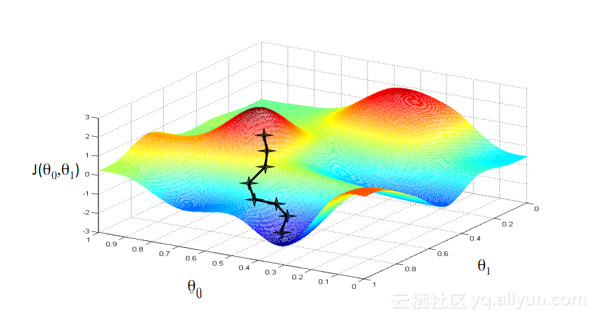
In the late 1990s, a major breakthrough solved the above-mentioned vanishing gradient problem and brought a second research boom to the development of RNN networks. The central idea of this big breakthrough is the introduction of unit long short-term memory (LSTM).
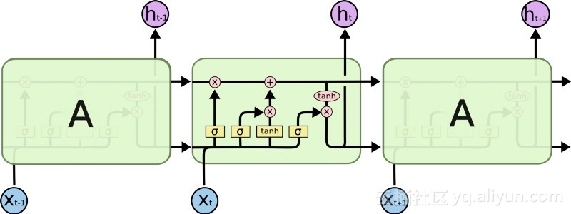
The introduction of LSTM has created a different world in the AI field. This is due to the fact that these new units or artificial neurons (like RNN’s standard short-term memory units) remember their inputs from the start. However, unlike standard RNN cells, LSTMs can be mounted on their memories, which have read/write properties similar to memory registers in regular computers. In addition, LSTMs are analog, not digital, making their features distinguishable. In other words, their curves are continuous and the steepness of their slopes can be found. Therefore, LSTM is particularly suitable for the partial calculus involved in backpropagation and gradient descent.
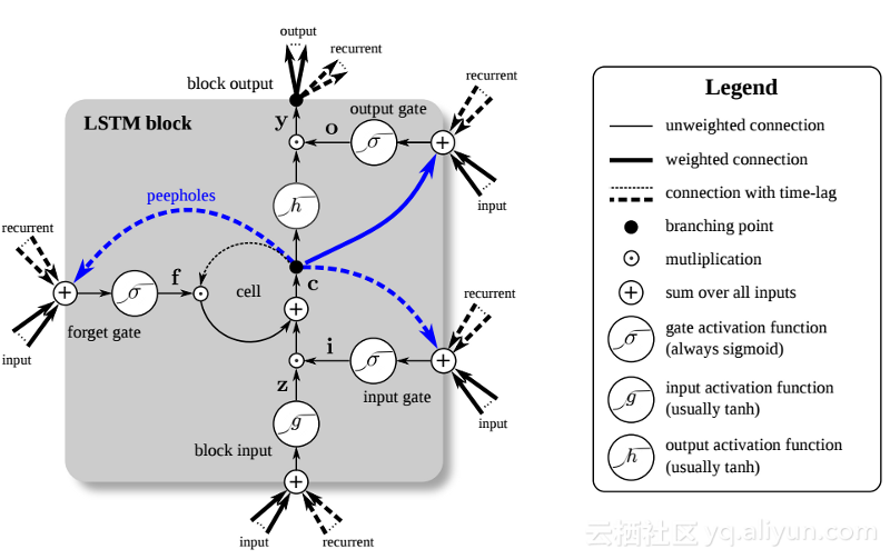
In summary, LSTM can not only adjust its weights, but also retain, delete, transform and control the inflow and outflow of its stored data based on the gradient of training. Most importantly, LSTM can preserve important error information for a long time so that the gradient is relatively steep and thus the training time of the network is relatively short. This solves the problem of vanishing gradients and greatly improves the accuracy of today’s LSTM-based RNN networks. Due to significant improvements in RNN architecture, Google, Apple, and many other advanced companies are now using RNN to power applications at the heart of their businesses.
Summarize Recurrent neural networks (RNN) can remember their previous inputs, giving them greater advantages than other artificial neural networks when it comes to continuous, context-sensitive tasks such as speech recognition.
Regarding the development history of RNN networks: The first generation of RNNs achieved the ability to correct errors through backpropagation and gradient descent algorithms. However, the vanishing gradient problem prevented the development of RNN; it was not until 1997 that a major breakthrough was achieved after the introduction of an LSTM-based architecture.
The new method effectively turns each unit in the RNN network into an analog computer, greatly improving network accuracy.
author information
Jason Roell: Software engineer with a passion for deep learning and its application to transformative technologies.
Linkedin: http://www.linkedin.com/in/jason-roell-47830817/
The above is the detailed content of Preferred Neural Networks for Application to Time Series Data. For more information, please follow other related articles on the PHP Chinese website!

Hot AI Tools

Undresser.AI Undress
AI-powered app for creating realistic nude photos

AI Clothes Remover
Online AI tool for removing clothes from photos.

Undress AI Tool
Undress images for free

Clothoff.io
AI clothes remover

AI Hentai Generator
Generate AI Hentai for free.

Hot Article

Hot Tools

Notepad++7.3.1
Easy-to-use and free code editor

SublimeText3 Chinese version
Chinese version, very easy to use

Zend Studio 13.0.1
Powerful PHP integrated development environment

Dreamweaver CS6
Visual web development tools

SublimeText3 Mac version
God-level code editing software (SublimeText3)

Hot Topics
 deepseek web version entrance deepseek official website entrance
Feb 19, 2025 pm 04:54 PM
DeepSeek is a powerful intelligent search and analysis tool that provides two access methods: web version and official website. The web version is convenient and efficient, and can be used without installation; the official website provides comprehensive product information, download resources and support services. Whether individuals or corporate users, they can easily obtain and analyze massive data through DeepSeek to improve work efficiency, assist decision-making and promote innovation.
 How to install deepseek
Feb 19, 2025 pm 05:48 PM
There are many ways to install DeepSeek, including: compile from source (for experienced developers) using precompiled packages (for Windows users) using Docker containers (for most convenient, no need to worry about compatibility) No matter which method you choose, Please read the official documents carefully and prepare them fully to avoid unnecessary trouble.
 Ouyi okx installation package is directly included
Feb 21, 2025 pm 08:00 PM
Ouyi OKX, the world's leading digital asset exchange, has now launched an official installation package to provide a safe and convenient trading experience. The OKX installation package of Ouyi does not need to be accessed through a browser. It can directly install independent applications on the device, creating a stable and efficient trading platform for users. The installation process is simple and easy to understand. Users only need to download the latest version of the installation package and follow the prompts to complete the installation step by step.
 BITGet official website installation (2025 beginner's guide)
Feb 21, 2025 pm 08:42 PM
BITGet is a cryptocurrency exchange that provides a variety of trading services including spot trading, contract trading and derivatives. Founded in 2018, the exchange is headquartered in Singapore and is committed to providing users with a safe and reliable trading platform. BITGet offers a variety of trading pairs, including BTC/USDT, ETH/USDT and XRP/USDT. Additionally, the exchange has a reputation for security and liquidity and offers a variety of features such as premium order types, leveraged trading and 24/7 customer support.
 Get the gate.io installation package for free
Feb 21, 2025 pm 08:21 PM
Gate.io is a popular cryptocurrency exchange that users can use by downloading its installation package and installing it on their devices. The steps to obtain the installation package are as follows: Visit the official website of Gate.io, click "Download", select the corresponding operating system (Windows, Mac or Linux), and download the installation package to your computer. It is recommended to temporarily disable antivirus software or firewall during installation to ensure smooth installation. After completion, the user needs to create a Gate.io account to start using it.
 Ouyi Exchange Download Official Portal
Feb 21, 2025 pm 07:51 PM
Ouyi, also known as OKX, is a world-leading cryptocurrency trading platform. The article provides a download portal for Ouyi's official installation package, which facilitates users to install Ouyi client on different devices. This installation package supports Windows, Mac, Android and iOS systems. Users can choose the corresponding version to download according to their device type. After the installation is completed, users can register or log in to the Ouyi account, start trading cryptocurrencies and enjoy other services provided by the platform.
 How to automatically set permissions of unixsocket after system restart?
Mar 31, 2025 pm 11:54 PM
How to automatically set the permissions of unixsocket after the system restarts. Every time the system restarts, we need to execute the following command to modify the permissions of unixsocket: sudo...
 Why does an error occur when installing an extension using PECL in a Docker environment? How to solve it?
Apr 01, 2025 pm 03:06 PM
Causes and solutions for errors when using PECL to install extensions in Docker environment When using Docker environment, we often encounter some headaches...


