Extend Q-Learning with Dyna-Q to enhance decision-making
Q-Learning is a crucial model-free algorithm in reinforcement learning that focuses on learning the value or "Q-value" of actions in a specific state. This approach works well in environments with unpredictability because it does not require a predefined model of the surrounding environment. It efficiently adapts to random transformations and various rewards, making it suitable for scenarios with uncertain outcomes. This flexibility makes Q-Learning a powerful tool for applications requiring adaptive decision-making without prior knowledge of environmental dynamics.

Extend Q-Learning with Dyna-Q to enhance decision-making
Explore Dyna-Q, This is an advanced reinforcement learning algorithm that extends Q-Learning by combining real-world experience with simulated planning.
Q-Learning is a crucial model-free algorithm in reinforcement learning that focuses on learning the value or "Q-value" of an action in a specific state. This approach works well in environments with unpredictability because it does not require a predefined model of the surrounding environment. It efficiently adapts to random transformations and various rewards, making it suitable for scenarios with uncertain outcomes. This flexibility makes Q-Learning a powerful tool for applications requiring adaptive decision-making without prior knowledge of environmental dynamics.
Learning Process
Q-learning works by updating the Q-value table for each action in each state. It uses the Bellman equation to iteratively update these values based on observed rewards and their estimates of future rewards. A policy - a strategy for choosing actions - is derived from these Q-values.
- Q value - represents the expected future reward that can be obtained by taking a specific action in a given state
- Update rules - Q value is updated as follows:
- Q ( state, action) ← Q (state, action) α (reward maximum γ Q (next state, a) − Q (state, action))
- The learning rate α represents the importance of new information, discount coefficient γ represents the importance of future rewards.
The code provided is used as the training function of Q-Learner. It utilizes the Bellman equation to determine the most efficient transitions between states.
def train_Q(self,s_prime,r):
        self.QTable[self.s,self.action] = (1-self.alpha)*self.QTable[self.s, self.action] + \
            self.alpha * (r + self.gamma * (self.QTable[s_prime, np.argmax(self.QTable[s_prime])]))
        self.experiences.append((self.s, self.action, s_prime, r))
        self.num_experiences = self.num_experiences + 1
        self.s = s_prime
        self.action = action
        return action
Exploration and Development
A key aspect of Q-learning is balancing exploration (trying new actions to discover their rewards) and exploitation (using known information to maximize rewards). Algorithms often use strategies such as ε-greedy to maintain this balance.
Start by setting the rate of random operations to balance exploration and exploitation. Implement a decay rate to gradually reduce randomness as the Q-table accumulates more data. This approach ensures that over time, as more evidence accumulates, the algorithm increasingly turns to exploiting.
if rand.random() >= self.random_action_rate:
  action = np.argmax(self.QTable[s_prime,:])  #Exploit: Select Action that leads to a State with the Best Reward
else:
  action = rand.randint(0,self.num_actions - 1) #Explore: Randomly select an Action.

# Use a decay rate to reduce the randomness (Exploration) as the Q-Table gets more evidence
self.random_action_rate = self.random_action_rate * self.random_action_decay_rate
Introducing Dyna-Q
Dyna-Q is an innovative extension of the traditional Q-Learning algorithm and is at the forefront of combining real-world experience with simulated planning. This approach significantly enhances the learning process by integrating actual interactions and simulated experiences, enabling agents to quickly adapt and make informed decisions in complex environments. By leveraging direct learning from environmental feedback and insights gained through simulation, Dyna-Q provides a comprehensive and effective strategy to address challenges where real-world data is scarce or costly to acquire.
Dyna-Q的组件
- Q-Learning:从真实经验中学习
- 模型学习:学习环境模型
- 规划:使用模型生成模拟体验
模型学习
- 该模型跟踪转换和奖励。对于每个状态-动作对 (s, a),模型存储下一个状态 s′ 和奖励 r。
- 当智能体观察到转换 (s, a,r,s′) 时,它会更新模型。
使用模拟体验进行规划
- 在每个步骤中,代理从真实体验更新其 Q 值后,还会根据模拟体验更新 Q 值。
- 这些体验是使用学习模型生成的:对于选定的状态-动作对(s,a),它预测下一个状态和奖励,并且Q值被更新,就好像已经经历了这种转变一样。
算法 Dyna-Q
- 初始化所有状态-动作对的 Q 值 Q(s, a) 和模型 (s, a)。
- 循环(每集):
- 初始化状态 s。
- 循环(针对剧集的每个步骤):
- 使用派生自 Q 从状态 s 中选择操作 a(例如,ε-greedy )
- 采取行动 a,观察奖励 r,然后下一个状态 s′
- 直接学习:使用观察到的跃迁(s、a、r、s′)更新 Q 值
- 模型学习:使用转换(s、a、r、s′)更新模型
- 计划:重复 n 次:
- 随机选择以前经历过的状态-动作对 (s, a)。
- 使用模型生成预测的下一个状态 s′ 并奖励 r
- 使用模拟跃迁 (s, a,r,s′) 更新 Q 值
- s← s′。
- 结束循环 此功能将 Dyna-Q 计划阶段合并到前面提到的 Q-Learner 中,从而能够指定在每一集中运行的所需模拟量,其中操作是随机选择的。此功能增强了 Q-Learn 的整体功能和多功能性。
def train_DynaQ(self,s_prime,r):
        self.QTable[self.s,self.action] = (1-self.alpha)*self.QTable[self.s, self.action] + \
            self.alpha * (r + self.gamma * (self.QTable[s_prime, np.argmax(self.QTable[s_prime])]))
        self.experiences.append((self.s, self.action, s_prime, r))
        self.num_experiences = self.num_experiences + 1

        # Dyna-Q Planning - Start
        if self.dyna_planning_steps > 0:  # Number of simulations to perform
            idx_array = np.random.randint(0, self.num_experiences, self.dyna)
            for exp in range(0, self.dyna): # Pick random experiences and update QTable
                idx = idx_array[exp]
                self.QTable[self.experiences[idx][0],self.experiences[idx][1]] = (1-self.alpha)*self.QTable[self.experiences[idx][0], self.experiences[idx][1]] + \
                    self.alpha * (self.experiences[idx][3] + self.gamma * (self.QTable[self.experiences[idx][2], np.argmax(self.QTable[self.experiences[idx][2],:])]))
        # Dyna-Q Planning - End

        if rand.random() >= self.random_action_rate:
          action = np.argmax(self.QTable[s_prime,:])  #Exploit: Select Action that leads to a State with the Best Reward
        else:
          action = rand.randint(0,self.num_actions - 1) #Explore: Randomly select an Action.

    	# Use a decay rate to reduce the randomness (Exploration) as the Q-Table gets more evidence
        self.random_action_rate = self.random_action_rate * self.random_action_decay_rate

        self.s = s_prime
        self.action = action
        return action
结论
Dyna Q 代表了一种进步,我们追求设计能够在复杂和不确定的环境中学习和适应的代理。通过理解和实施 Dyna Q,人工智能和机器学习领域的专家和爱好者可以为各种实际问题设计出有弹性的解决方案。本教程的目的不是介绍概念和算法,而是在这个引人入胜的研究领域激发创造性应用和未来进展的创造力。
The above is the detailed content of Extend Q-Learning with Dyna-Q to enhance decision-making. For more information, please follow other related articles on the PHP Chinese website!

Hot AI Tools

Undresser.AI Undress
AI-powered app for creating realistic nude photos

AI Clothes Remover
Online AI tool for removing clothes from photos.

Undress AI Tool
Undress images for free

Clothoff.io
AI clothes remover

AI Hentai Generator
Generate AI Hentai for free.

Hot Article

Hot Tools

Notepad++7.3.1
Easy-to-use and free code editor

SublimeText3 Chinese version
Chinese version, very easy to use

Zend Studio 13.0.1
Powerful PHP integrated development environment

Dreamweaver CS6
Visual web development tools

SublimeText3 Mac version
God-level code editing software (SublimeText3)

Hot Topics
 1376
1376
 52
52
 I Tried Vibe Coding with Cursor AI and It's Amazing!
Mar 20, 2025 pm 03:34 PM
Vibe coding is reshaping the world of software development by letting us create applications using natural language instead of endless lines of code. Inspired by visionaries like Andrej Karpathy, this innovative approach lets dev
 Top 5 GenAI Launches of February 2025: GPT-4.5, Grok-3 & More!
Mar 22, 2025 am 10:58 AM
February 2025 has been yet another game-changing month for generative AI, bringing us some of the most anticipated model upgrades and groundbreaking new features. From xAI’s Grok 3 and Anthropic’s Claude 3.7 Sonnet, to OpenAI’s G
 How to Use YOLO v12 for Object Detection?
Mar 22, 2025 am 11:07 AM
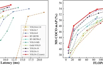
YOLO (You Only Look Once) has been a leading real-time object detection framework, with each iteration improving upon the previous versions. The latest version YOLO v12 introduces advancements that significantly enhance accuracy
 Is ChatGPT 4 O available?
Mar 28, 2025 pm 05:29 PM
ChatGPT 4 is currently available and widely used, demonstrating significant improvements in understanding context and generating coherent responses compared to its predecessors like ChatGPT 3.5. Future developments may include more personalized interactions and real-time data processing capabilities, further enhancing its potential for various applications.
 Google's GenCast: Weather Forecasting With GenCast Mini Demo
Mar 16, 2025 pm 01:46 PM
Google DeepMind's GenCast: A Revolutionary AI for Weather Forecasting Weather forecasting has undergone a dramatic transformation, moving from rudimentary observations to sophisticated AI-powered predictions. Google DeepMind's GenCast, a groundbreak
 Which AI is better than ChatGPT?
Mar 18, 2025 pm 06:05 PM
The article discusses AI models surpassing ChatGPT, like LaMDA, LLaMA, and Grok, highlighting their advantages in accuracy, understanding, and industry impact.(159 characters)
 o1 vs GPT-4o: Is OpenAI's New Model Better Than GPT-4o?
Mar 16, 2025 am 11:47 AM
OpenAI's o1: A 12-Day Gift Spree Begins with Their Most Powerful Model Yet December's arrival brings a global slowdown, snowflakes in some parts of the world, but OpenAI is just getting started. Sam Altman and his team are launching a 12-day gift ex
 Best AI Art Generators (Free & Paid) for Creative Projects
Apr 02, 2025 pm 06:10 PM
The article reviews top AI art generators, discussing their features, suitability for creative projects, and value. It highlights Midjourney as the best value for professionals and recommends DALL-E 2 for high-quality, customizable art.


