
One of the common problems is that the values in cells D3 to D6 are text values, which may cause some errors. The solution is to change the values of these cells to regular values so that they can run normally. Hope this little tip can help everyone!
The formula can be written as
=AVERAGE(D3:D6)
How to convert text directly into numerical values?
method one
In order to solve the problem of text formatting values in a large number of cells, we can take the following method: select the cell, right-click, select "Format Cells", change the format from "Text" to "General", and then press Press the Enter key to confirm. However, this approach can be very inconvenient if there are a large number of cells that need to be changed.
Method Two
To convert the selected cells or range of cells to regular numbers, you can follow the steps below: 1. Select an empty cell. 2. Right-click the selected cell and select "Copy". 3. Select the cell and cell range where the text format is located again. 4. Right-click the selected cells and cell range and select "Paste Special". 5. Select "Add" from the pop-up options, and then click "OK". Through the above steps, you can add 0 to the selected cell or range of cells to convert it into a regular number. This will solve the problem.
Method 3
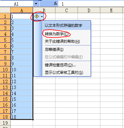
Select the cell or cell range where the text format value is located------an option icon will appear next to the selected cell or cell range----click and the option menu will appear----Select "Convert to numbers"
Method 4
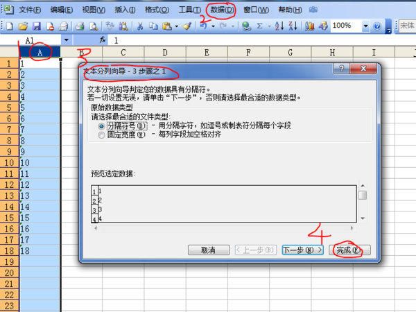
Select the column that is in text format----data----separate into columns----complete---right-click again---set the cell format to normal---confirm
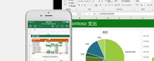
You can select all the data that require average value, then click on the toolbar above the software, then pull down the toolbar and select [Average]; you can also insert the [AVERAGE] function in the cell and enter the cell that needs to be calculated. area, click OK. The specific instructions are as follows:
1. Method 1: Use the average value of the built-in tool
1. In EXCEL average, select the data to be calculated in the table;
2. Click on the toolbar above the software, you will see the buttons with and, then directly click on the drop-down menu and select [Average];
3. Finally, the software will automatically fill in the average value of all data to the end of this column of data;
2. Method 2: Use function to get the average value
1. Position the mouse in the cell where you want to enter the function, then select [Formula] in the menu bar, and select [Insert Function] in the common menu bar;
2. In the pop-up Insert Function dialog box, find the [AVERAGE] function in the function and click [OK];
3. At this time, we set the function parameters, select the cells that need to calculate the average value, and click [OK] when the settings are completed;
4. If we need to calculate the average of multiple rows of data, we can position the mouse at the lower right corner of the cell where the average is calculated, and drag down when the cursor turns into a black number.
1. First we open the excel spreadsheet to be edited;
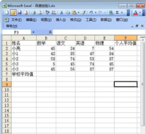
2. Select the value of the average value you want to calculate. You can first select a column or a row. Here I select all;
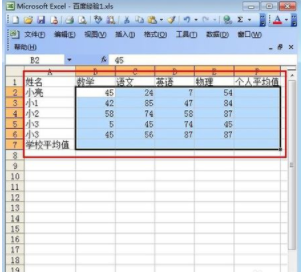
3. Click the function calculation icon in the menu bar;
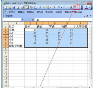
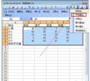
4Click "Average" inside;
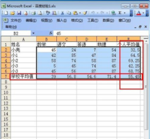
5. After completing the above steps, you can calculate the average value you want;
Extended information
Function Encyclopedia
Database and inventory management functions
AVERAGE Returns the average value of selected database items
COUNT Counts the number of cells containing numbers in the database
COUNTA calculates the number of non-empty cells in the database
DGET Extracts a single record that meets the specified conditions from the database
MAX Returns the maximum value in the selected database item
MIN Returns the minimum value in the selected database item
PRODUCT Multiplies the value in a specific field (the records in this field are the records in the database that meet the specified conditions)
STDEV Estimates the standard deviation based on samples of selected items in the database
STDEVP Calculates the standard deviation based on the sample population of selected items in the database
SUM sums the numbers in the field columns of the records in the database that meet the conditions
VAR estimates variance based on examples of selected items in the database
VARP calculates the variance based on the sample population of selected items in the database
GETPIVOTDATA Returns the data stored in the PivotTable report
Reference material: Sogou Encyclopedia: excel function
There are two types:
=average()
Return the average value (arithmetic mean) of the parameters.
grammar
AVERAGE(number1,number2,...)
Number1, number2, ...
is 1 to 30 parameters that need to be calculated.
illustrate
The parameter can be a number, or a name, array, or reference containing a number.
If the array or reference parameter contains text, logical values, or blank cells, these values will be ignored; however, cells containing zero values will be counted.
hint
When averaging values in cells, you should keep in mind the difference between blank cells and cells with zero values, especially if "Zero Values" has been cleared on the "View" tab in the "Options" dialog box. For checkbox conditions, blank cells are not counted, but zero values are counted. To view the Options dialog box, click Options on the Tools menu.
Example
The example may be easier to understand if you copy it into a blank worksheet.
How to operate
Create a blank workbook or worksheet.
Please select an example in the Help topic. Do not select row or column headers.
Choose an example from the help.
Press Ctrl C.
In the worksheet, select cell A1 and press Ctrl V.
To switch between viewing results and viewing the formula that returns the results, press Ctrl ` (accent accent), or on the Tools menu, point to Formula Audit, and then click Formula Audit Mode.
1
2
3
4
5
6
A
data
10
7
9
27
2
Formula Description (Result)
=AVERAGE(A2:A6) The average of the above numbers (11)
=AVERAGE(A2:A6, 5) The average of the above number and 5 (10)
=trimmean()
TRIMMEAN
Please refer to
Returns the internal average of the data set. The function TRIMMEAN removes a percentage of data points from the head and tail of the data set and then averages them. You can use this function when you want to exclude calculations on a portion of the data from your analysis.
grammar
TRIMMEAN(array,percent)
Array
is the array or numerical area that needs to be sorted and averaged.
Percent
is the proportion of data points to be removed during calculation. For example, if percentage = 0.2, in a set of 20 data points, 4 data points (20 x 0.2) will be removed: 2 from the head and 2 from the tail. Remove 2.
illustrate
If percent 1, function TRIMMEAN returns the error value #NUM!.
Function TRIMMEAN rounds down the number of data points to remove to the nearest multiple of 2. If percent = 0.1, 10% of 30 data points equals 3 data points. The function TRIMMEAN will symmetrically remove one item from the head and one item from the tail of the data set.
Example
The example may be easier to understand if you copy it into a blank worksheet.
How to operate
Create a blank workbook or worksheet.
Please select an example in the Help topic. Do not select row or column headers.
Choose an example from the help.
Press Ctrl C.
In the worksheet, select cell A1 and press Ctrl V.
To switch between viewing results and viewing the formula that returns the results, press Ctrl ` (accent accent), or on the Tools menu, point to Formula Audit, and then click Formula Audit Mode.
1
2
3
4
5
6
7
8
9
10
11
12
A
data
4
5
6
7
2
3
4
5
1
2
3
Formula Description (Result)
=TRIMMEAN(A2:A12,0.2) Internal mean of the above data set (remove 20% from calculation) (3.777778)
The above is the detailed content of Calculate the average of data using Excel. For more information, please follow other related articles on the PHP Chinese website!
 What software is zoom?
 MySQL index
 Why is there no signal on the monitor after turning on the computer?
 The role of base tag
 Introduction to hard disk interface types
 How to use googlevoice
 The difference between JD.com's self-operated flagship store and its official flagship store
 What does Matcha Exchange do?


