Implementing noise removal diffusion model using PyTorch
Before understanding the working principle of the Denoising Diffusion Probability Model (DDPM) in detail, let’s first understand some of the development of generative artificial intelligence, which is also one of the basic research of DDPM.

VAE
VAE uses an encoder, a probabilistic latent space and a decoder. During training, the encoder predicts the mean and variance of each image and samples these values from a Gaussian distribution. The result of the sampling is passed to the decoder, which converts the input image into a form similar to the output image. KL divergence is used to calculate the loss. A significant advantage of VAE is its ability to generate diverse images. In the sampling stage, one can directly sample from the Gaussian distribution and generate new images through the decoder.
GAN
Just one year after variational autoencoders (VAEs), a groundbreaking family of generative models has emerged. — Generative Adversarial Networks (GANs), marking the beginning of a new class of generative models, characterized by the collaboration of two neural networks: a generator and a discriminator, involving an adversarial training process. The goal of the generator is to generate real data, such as images, from random noise, while the discriminator strives to distinguish real data from generated data. Throughout the training phase, the generator and discriminator continuously improve their abilities through a competitive learning process. The generator generates increasingly convincing data, thereby becoming smarter than the discriminator, which in turn improves its ability to distinguish between real and generated samples. This adversarial interplay culminates in the generator producing high-quality, realistic data. In the sampling stage, after GAN training, the generator generates new samples by inputting random noise. It converts this noise into data that generally reflects real examples.
Why we need another model architecture
Although GANs and VAEs have their own advantages in image generation, they both have some problems. GANs can generate realistic images that are very similar to the images in the training set, but their generated results lack diversity. VAEs can create a variety of images, but tend to produce blurry images. However, there has been no success in combining these two capabilities to create images that are both highly realistic and diverse. This challenge represents a significant obstacle for researchers and needs to be addressed. Therefore, one of the future research directions is to explore how to combine the advantages of GANs and VAEs to achieve highly realistic and diverse image generation. This will bring a major breakthrough in the field of image generation and be widely used in various fields.
Six years after the publication of the GAN paper and seven years after the publication of the VAE paper, a groundbreaking model emerged, namely the denoising diffusion probability model (DDPM). DDPM combines the advantages of both fields to create diverse and realistic images.
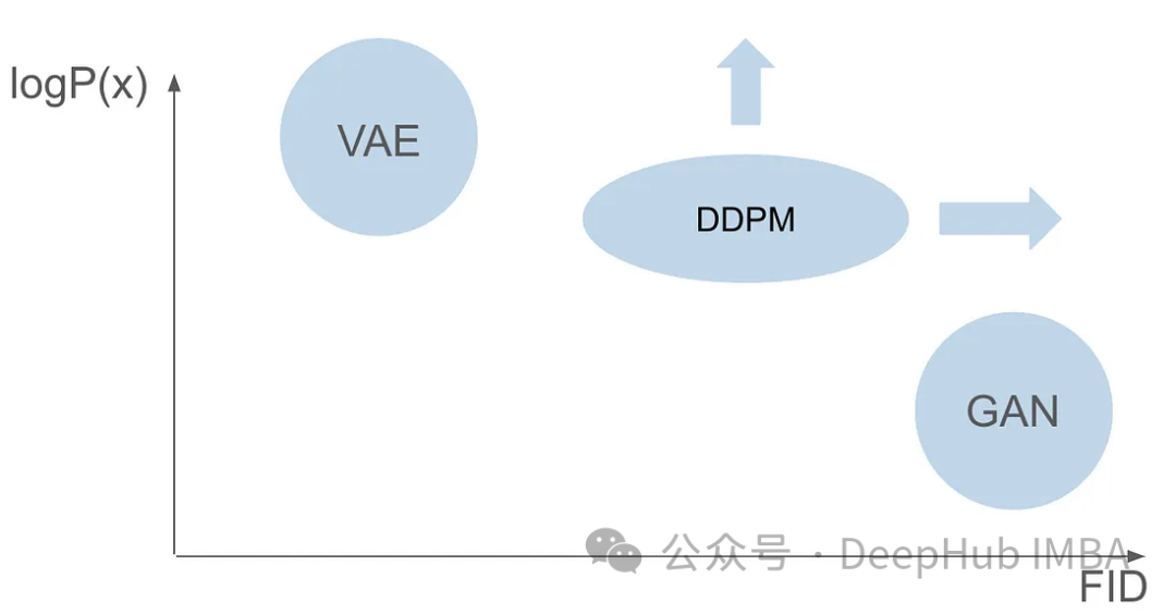
This article will explore the complexity of DDPM in detail, including the training process, forward and reverse processes, and sampling methods. We will use PyTorch to build and train DDPM from scratch, guiding readers through the entire process.
It is assumed that you are already familiar with the basic knowledge of deep learning and have a solid foundation in deep computer vision. We will not go into detail about these basic concepts, but instead aim to generate images that are believable in their authenticity.
DDPM
Denoising Diffusion Probabilistic Model (DDPM) is a cutting-edge method in the field of generative models. Compared with traditional models that rely on explicit likelihood functions, DDPM operates through an iterative denoising diffusion process. This process involves gradually adding noise to an image and trying to remove that noise. The basic theory is based on the idea of converting a simple distribution (such as a Gaussian distribution) into a complex and expressive image data distribution through a series of diffusion steps. In other words, by transferring samples from the original image distribution to a Gaussian distribution, we can build a model to reverse this process. This allows us to start from a fully Gaussian distribution and generate new images with image distribution characteristics, thus achieving efficient image generation.
The training of DDPM consists of two basic steps: the forward process that generates noisy images which is fixed and unlearnable, and the subsequent reverse process. The main goal of the inverse process is to denoise images using specialized machine learning models.
Forward Diffusion Process
The forward process is a fixed and non-learnable step, but it requires some predefined settings. Before we dive into the settings, let's first understand how it works.
The core concept of this process is to start with a clear image. At a specific step size, denoted by "T", a small amount of noise is gradually introduced following a Gaussian distribution.

As can be seen from the image, the noise is increasing at each step. Let's delve into the mathematical representation of this noise.
Noise is sampled from a Gaussian distribution. To introduce a small amount of noise at each step, we use a Markov chain. To generate an image of the current timestamp, we only need an image of the last timestamp. The concept of Markov chains is key here and will be crucial to the mathematical details that follow.
A Markov chain is a stochastic process in which the probability of transition to any particular state depends only on the current state and elapsed time, not on the previous sequence of events. This feature simplifies the modeling of the noise addition process, making it easier to analyze mathematically.

The variance parameter, expressed as beta, is intentionally set to a very small value in order to introduce only the minimum amount at each step noise.
The step parameter "T" determines the step size required to generate a fully noisy image. In this article, this parameter is set to 1000, which may seem large. Do we really need to create 1000 noisy images for every original image in the dataset? The Markov chain aspect is proven to help solve this problem. Since we only need the image from the previous step to predict the next step, and the noise added at each step remains the same, we can simplify the calculation by generating noisy images at specific timestamps. Employing a pair reparameterization technique allows us to further simplify the equations.

Incorporate the new parameters introduced in Equation (3) into Equation (2), develop Equation (2), and obtain the result .
Inverse Diffusion Process
We have introduced noise to the image and the next step is to perform the inverse operation. Unless we know the initial conditions, i.e. the undenoised image at t = 0, it is impossible to mathematically implement the reverse process to denoise the image. Our goal is to sample directly from noise to create new images, and here there is a lack of information about the results. So I need to devise a way to progressively denoise an image without knowing the result. So the solution came to use deep learning models to approximate this complex mathematical function.
With a little mathematical background, the model will approximate equation (5). One detail worth noting is that we will stick to the original DDPM paper and keep the variance fixed, although it is also possible to make the model learn it.

The model is tasked with predicting the average of the noise added between the current timestamp and the previous timestamp. This can effectively remove noise and achieve the desired effect. But what if our goal is to have the model predict the noise added from the "original image" to the last timestamp?
Unless we know the initial image without noise, it is mathematically impossible to perform The reverse process is challenging, let's start by defining the posterior variance.
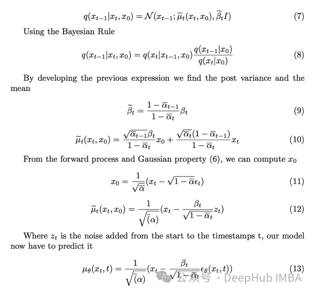
#The task of the model is to predict the noise added to the image at timestamp t from the initial image. The forward process allows us to perform this operation, starting with a clear image and progressing to a noisy image at timestamp t.
Training Algorithm
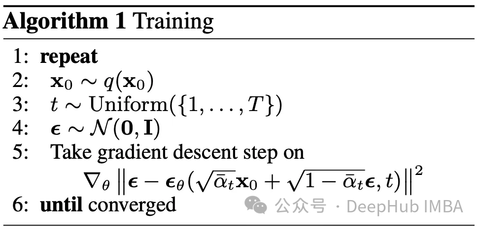
We assume that the model architecture used to make predictions will be a U-Net. The goal of the training phase is: for each image in the dataset, randomly select a timestamp in the range [0, T] and calculate the forward diffusion process. This produces a clear, somewhat noisy image, as well as the actual noise used. This model is then used to predict the noise added to the image using our understanding of the inverse process. With real and predicted noise, we appear to have entered a supervised machine learning problem.
The most important question is, which loss function should we use to train our model? Since we are dealing with the probabilistic latent space, the Kullback-Leibler (KL) divergence is a Suitable choice.
KL divergence measures the difference between two probability distributions, in our case, the distribution predicted by the model and the expected distribution. Incorporating KL divergence into the loss function not only guides the model to produce accurate predictions, but also ensures that the latent space representation conforms to the desired probability structure.
KL divergence can be approximated as the L2 loss function, so the following loss function can be obtained:

## Finally we got the training algorithm proposed in the paper.
Sampling
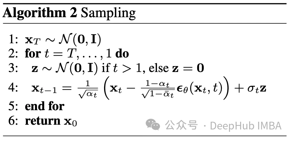
The reverse process has been explained, here is how to use it. Starting from a completely random image at time T, and using the reverse process T times, we finally reach time 0. This forms the second algorithm outlined in this article
Parameters
We have many different Parameters beta, beta_tildes, alpha, alpha_hat, etc. I still don't know how to choose these parameters. But the only parameter known at this point is T, which is set to 1000.
For all listed parameters, their selection depends on the beta. In a sense, Beta determines the amount of noise we want to add at each step. Therefore, to ensure the success of the algorithm, careful beta selection is crucial. Because there are too many other parameters, please refer to the paper.
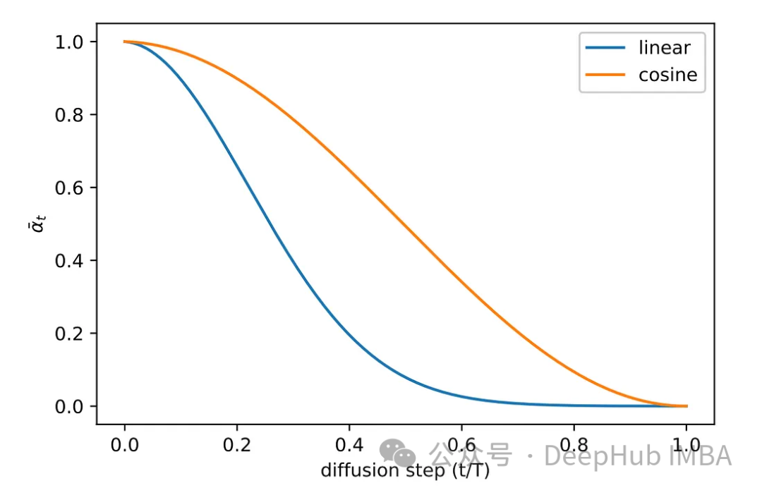
Various sampling methods were explored during the experimental phase of the original paper. The original linear sampling method images either received insufficient noise or became too noisy. To solve this problem, another more common method is adopted, namely cosine sampling. Cosine sampling provides smoother and more consistent noise addition.
Model Pytorch implementation
We will use the U-Net architecture for noise prediction, the reason for choosing U-Net, because U-Net is an ideal architecture for image processing, capturing spatial and feature maps, and providing the same output size as the input.
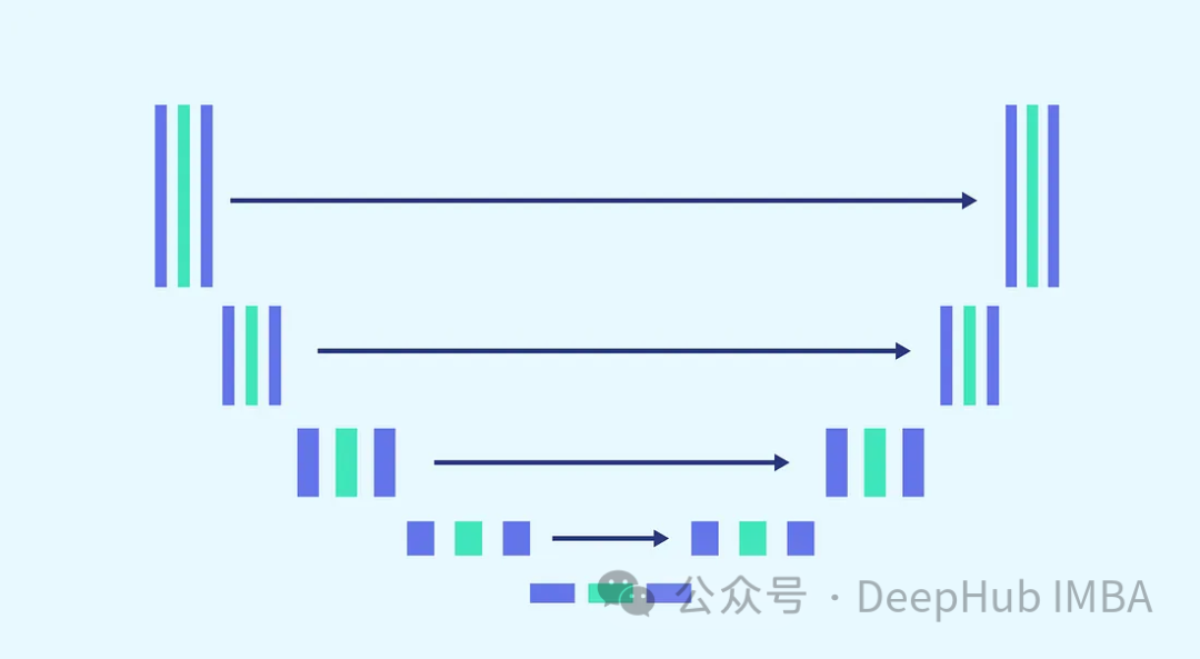
Taking into account the complexity of the task and the requirement to use the same model for each step (where the model needs to be able to denoise with the same weights as completely noisy images and slightly noisy images), adjusting the model is essential. This includes merging more complex blocks and introducing awareness of the timestamps used via a sinusoidal embedding step. The purpose of these enhancements is to make the model an expert in denoising tasks. We will introduce each block before moving on to build the complete model.
ConvNext block
In order to meet the need to increase model complexity, the convolution block plays a vital role. We cannot just rely on the basic blocks in the u-net paper here, we will combine it with ConvNext.
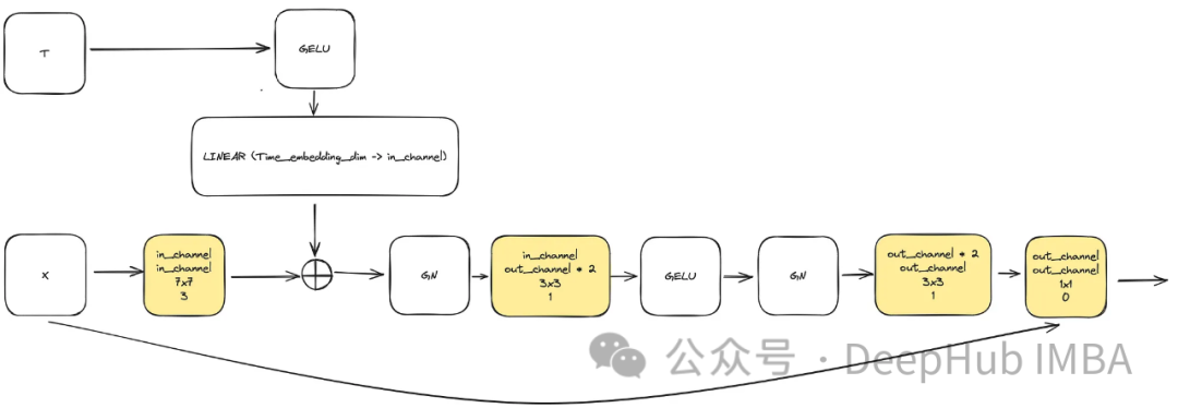
The input consists of an "x" representing an image and an embedded timestamp visualization "t" of size "time_embedding_dim". Throughout the process, blocks play a key role in learning spatial and feature maps due to their complexity and residual connections to the input and final layer.
class ConvNextBlock(nn.Module):def __init__(self,in_channels,out_channels,mult=2,time_embedding_dim=None,norm=True,group=8,):super().__init__()self.mlp = (nn.Sequential(nn.GELU(), nn.Linear(time_embedding_dim, in_channels))if time_embedding_dimelse None) self.in_conv = nn.Conv2d(in_channels, in_channels, 7, padding=3, groups=in_channels) self.block = nn.Sequential(nn.GroupNorm(1, in_channels) if norm else nn.Identity(),nn.Conv2d(in_channels, out_channels * mult, 3, padding=1),nn.GELU(),nn.GroupNorm(1, out_channels * mult),nn.Conv2d(out_channels * mult, out_channels, 3, padding=1),) self.residual_conv = (nn.Conv2d(in_channels, out_channels, 1)if in_channels != out_channelselse nn.Identity()) def forward(self, x, time_embedding=None):h = self.in_conv(x)if self.mlp is not None and time_embedding is not None:assert self.mlp is not None, "MLP is None"h = h + rearrange(self.mlp(time_embedding), "b c -> b c 1 1")h = self.block(h)return h + self.residual_conv(x)
Sinusoidal timestamp embedding
One of the key blocks in the model is the sinusoidal timestamp embedding block, which makes the The encoding is able to retain information about the current time required for the model to be decoded, as the model will be used for all different timestamps.
This is a very classic implementation and is used in various places. We will paste the code directly
class SinusoidalPosEmb(nn.Module):def __init__(self, dim, theta=10000):super().__init__()self.dim = dimself.theta = theta def forward(self, x):device = x.devicehalf_dim = self.dim // 2emb = math.log(self.theta) / (half_dim - 1)emb = torch.exp(torch.arange(half_dim, device=device) * -emb)emb = x[:, None] * emb[None, :]emb = torch.cat((emb.sin(), emb.cos()), dim=-1)return emb
DownSample & UpSample
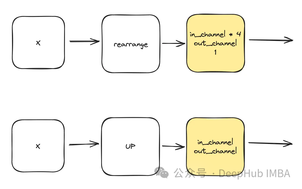
class DownSample(nn.Module):def __init__(self, dim, dim_out=None):super().__init__()self.net = nn.Sequential(Rearrange("b c (h p1) (w p2) -> b (c p1 p2) h w", p1=2, p2=2),nn.Conv2d(dim * 4, default(dim_out, dim), 1),) def forward(self, x):return self.net(x) class Upsample(nn.Module):def __init__(self, dim, dim_out=None):super().__init__()self.net = nn.Sequential(nn.Upsample(scale_factor=2, mode="nearest"),nn.Conv2d(dim, dim_out or dim, kernel_size=3, padding=1),) def forward(self, x):return self.net(x)Temporal multi-layer perceptron
This module utilizes it to calculate the time based on the given timestamp t Creation time representation. The output of this multilayer perceptron (MLP) will also serve as the input "t" to all modified ConvNext blocks.

Here, "dim" is a hyperparameter of the model, indicating the number of channels required for the first block. It serves as the base calculation for the number of channels in subsequent blocks.
sinu_pos_emb = SinusoidalPosEmb(dim, theta=10000) time_dim = dim * 4 time_mlp = nn.Sequential(sinu_pos_emb,nn.Linear(dim, time_dim),nn.GELU(),nn.Linear(time_dim, time_dim),)
Attention
This is an optional component used in unet. Attention helps enhance the role of residual connections in learning. It pays more attention to the important spatial information obtained from the left side of Unet through the attention mechanism calculated by residual connections and the feature map calculated by medium and low latent spaces. It comes from the ACC-UNet paper.
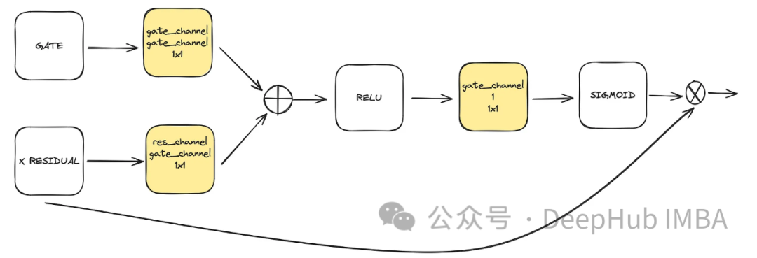
gate represents the upsampled output of the lower block, while x-residual represents the residual connection at the level where attention is applied.
class BlockAttention(nn.Module):def __init__(self, gate_in_channel, residual_in_channel, scale_factor):super().__init__()self.gate_conv = nn.Conv2d(gate_in_channel, gate_in_channel, kernel_size=1, stride=1)self.residual_conv = nn.Conv2d(residual_in_channel, gate_in_channel, kernel_size=1, stride=1)self.in_conv = nn.Conv2d(gate_in_channel, 1, kernel_size=1, stride=1)self.relu = nn.ReLU()self.sigmoid = nn.Sigmoid() def forward(self, x: torch.Tensor, g: torch.Tensor) -> torch.Tensor:in_attention = self.relu(self.gate_conv(g) + self.residual_conv(x))in_attention = self.in_conv(in_attention)in_attention = self.sigmoid(in_attention)return in_attention * x
最后整合
将前面讨论的所有块(不包括注意力块)整合到一个Unet中。每个块都包含两个残差连接,而不是一个。这个修改是为了解决潜在的过度拟合问题。
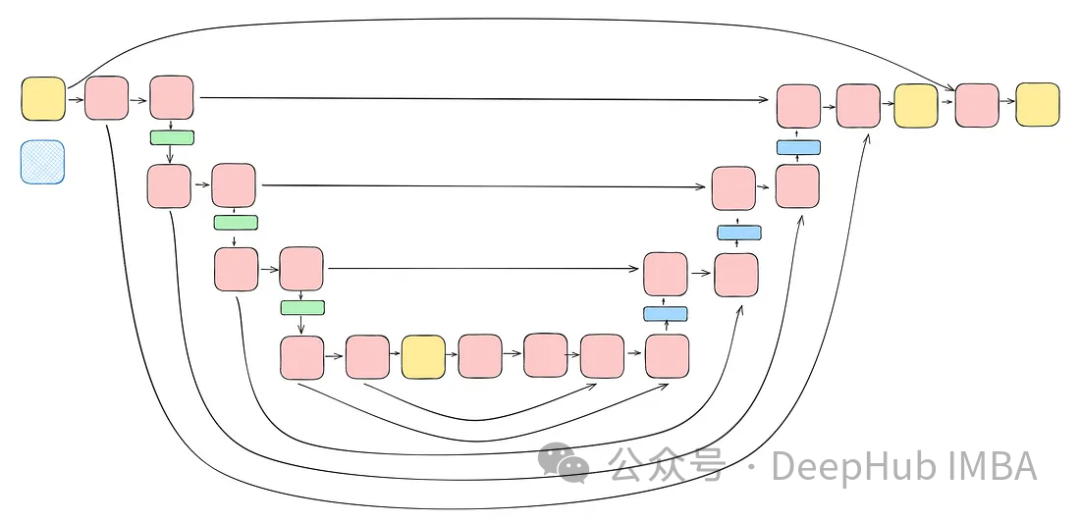
class TwoResUNet(nn.Module):def __init__(self,dim,init_dim=None,out_dim=None,dim_mults=(1, 2, 4, 8),channels=3,sinusoidal_pos_emb_theta=10000,convnext_block_groups=8,):super().__init__()self.channels = channelsinput_channels = channelsself.init_dim = default(init_dim, dim)self.init_conv = nn.Conv2d(input_channels, self.init_dim, 7, padding=3) dims = [self.init_dim, *map(lambda m: dim * m, dim_mults)]in_out = list(zip(dims[:-1], dims[1:])) sinu_pos_emb = SinusoidalPosEmb(dim, theta=sinusoidal_pos_emb_theta) time_dim = dim * 4 self.time_mlp = nn.Sequential(sinu_pos_emb,nn.Linear(dim, time_dim),nn.GELU(),nn.Linear(time_dim, time_dim),) self.downs = nn.ModuleList([])self.ups = nn.ModuleList([])num_resolutions = len(in_out) for ind, (dim_in, dim_out) in enumerate(in_out):is_last = ind >= (num_resolutions - 1) self.downs.append(nn.ModuleList([ConvNextBlock(in_channels=dim_in,out_channels=dim_in,time_embedding_dim=time_dim,group=convnext_block_groups,),ConvNextBlock(in_channels=dim_in,out_channels=dim_in,time_embedding_dim=time_dim,group=convnext_block_groups,),DownSample(dim_in, dim_out)if not is_lastelse nn.Conv2d(dim_in, dim_out, 3, padding=1),])) mid_dim = dims[-1]self.mid_block1 = ConvNextBlock(mid_dim, mid_dim, time_embedding_dim=time_dim)self.mid_block2 = ConvNextBlock(mid_dim, mid_dim, time_embedding_dim=time_dim) for ind, (dim_in, dim_out) in enumerate(reversed(in_out)):is_last = ind == (len(in_out) - 1)is_first = ind == 0 self.ups.append(nn.ModuleList([ConvNextBlock(in_channels=dim_out + dim_in,out_channels=dim_out,time_embedding_dim=time_dim,group=convnext_block_groups,),ConvNextBlock(in_channels=dim_out + dim_in,out_channels=dim_out,time_embedding_dim=time_dim,group=convnext_block_groups,),Upsample(dim_out, dim_in)if not is_lastelse nn.Conv2d(dim_out, dim_in, 3, padding=1)])) default_out_dim = channelsself.out_dim = default(out_dim, default_out_dim) self.final_res_block = ConvNextBlock(dim * 2, dim, time_embedding_dim=time_dim)self.final_conv = nn.Conv2d(dim, self.out_dim, 1) def forward(self, x, time):b, _, h, w = x.shapex = self.init_conv(x)r = x.clone() t = self.time_mlp(time) unet_stack = []for down1, down2, downsample in self.downs:x = down1(x, t)unet_stack.append(x)x = down2(x, t)unet_stack.append(x)x = downsample(x) x = self.mid_block1(x, t)x = self.mid_block2(x, t) for up1, up2, upsample in self.ups:x = torch.cat((x, unet_stack.pop()), dim=1)x = up1(x, t)x = torch.cat((x, unet_stack.pop()), dim=1)x = up2(x, t)x = upsample(x) x = torch.cat((x, r), dim=1)x = self.final_res_block(x, t) return self.final_conv(x)
扩散的代码实现
最后我们介绍一下扩散是如何实现的。由于我们已经介绍了用于正向、逆向和采样过程的所有数学理论,所里这里将重点介绍代码。
class DiffusionModel(nn.Module):SCHEDULER_MAPPING = {"linear": linear_beta_schedule,"cosine": cosine_beta_schedule,"sigmoid": sigmoid_beta_schedule,} def __init__(self,model: nn.Module,image_size: int,*,beta_scheduler: str = "linear",timesteps: int = 1000,schedule_fn_kwargs: dict | None = None,auto_normalize: bool = True,) -> None:super().__init__()self.model = model self.channels = self.model.channelsself.image_size = image_size self.beta_scheduler_fn = self.SCHEDULER_MAPPING.get(beta_scheduler)if self.beta_scheduler_fn is None:raise ValueError(f"unknown beta schedule {beta_scheduler}") if schedule_fn_kwargs is None:schedule_fn_kwargs = {} betas = self.beta_scheduler_fn(timesteps, **schedule_fn_kwargs)alphas = 1.0 - betasalphas_cumprod = torch.cumprod(alphas, dim=0)alphas_cumprod_prev = F.pad(alphas_cumprod[:-1], (1, 0), value=1.0)posterior_variance = (betas * (1.0 - alphas_cumprod_prev) / (1.0 - alphas_cumprod)) register_buffer = lambda name, val: self.register_buffer(name, val.to(torch.float32)) register_buffer("betas", betas)register_buffer("alphas_cumprod", alphas_cumprod)register_buffer("alphas_cumprod_prev", alphas_cumprod_prev)register_buffer("sqrt_recip_alphas", torch.sqrt(1.0 / alphas))register_buffer("sqrt_alphas_cumprod", torch.sqrt(alphas_cumprod))register_buffer("sqrt_one_minus_alphas_cumprod", torch.sqrt(1.0 - alphas_cumprod))register_buffer("posterior_variance", posterior_variance) timesteps, *_ = betas.shapeself.num_timesteps = int(timesteps) self.sampling_timesteps = timesteps self.normalize = normalize_to_neg_one_to_one if auto_normalize else identityself.unnormalize = unnormalize_to_zero_to_one if auto_normalize else identity @torch.inference_mode()def p_sample(self, x: torch.Tensor, timestamp: int) -> torch.Tensor:b, *_, device = *x.shape, x.devicebatched_timestamps = torch.full((b,), timestamp, device=device, dtype=torch.long) preds = self.model(x, batched_timestamps) betas_t = extract(self.betas, batched_timestamps, x.shape)sqrt_recip_alphas_t = extract(self.sqrt_recip_alphas, batched_timestamps, x.shape)sqrt_one_minus_alphas_cumprod_t = extract(self.sqrt_one_minus_alphas_cumprod, batched_timestamps, x.shape) predicted_mean = sqrt_recip_alphas_t * (x - betas_t * preds / sqrt_one_minus_alphas_cumprod_t) if timestamp == 0:return predicted_meanelse:posterior_variance = extract(self.posterior_variance, batched_timestamps, x.shape)noise = torch.randn_like(x)return predicted_mean + torch.sqrt(posterior_variance) * noise @torch.inference_mode()def p_sample_loop(self, shape: tuple, return_all_timesteps: bool = False) -> torch.Tensor:batch, device = shape[0], "mps" img = torch.randn(shape, device=device)# This cause me a RunTimeError on MPS device due to MPS back out of memory# No ideas how to resolve it at this point # imgs = [img] for t in tqdm(reversed(range(0, self.num_timesteps)), total=self.num_timesteps):img = self.p_sample(img, t)# imgs.append(img) ret = img # if not return_all_timesteps else torch.stack(imgs, dim=1) ret = self.unnormalize(ret)return ret def sample(self, batch_size: int = 16, return_all_timesteps: bool = False) -> torch.Tensor:shape = (batch_size, self.channels, self.image_size, self.image_size)return self.p_sample_loop(shape, return_all_timesteps=return_all_timesteps) def q_sample(self, x_start: torch.Tensor, t: int, noise: torch.Tensor = None) -> torch.Tensor:if noise is None:noise = torch.randn_like(x_start) sqrt_alphas_cumprod_t = extract(self.sqrt_alphas_cumprod, t, x_start.shape)sqrt_one_minus_alphas_cumprod_t = extract(self.sqrt_one_minus_alphas_cumprod, t, x_start.shape) return sqrt_alphas_cumprod_t * x_start + sqrt_one_minus_alphas_cumprod_t * noise def p_loss(self,x_start: torch.Tensor,t: int,noise: torch.Tensor = None,loss_type: str = "l2",) -> torch.Tensor:if noise is None:noise = torch.randn_like(x_start)x_noised = self.q_sample(x_start, t, noise=noise)predicted_noise = self.model(x_noised, t) if loss_type == "l2":loss = F.mse_loss(noise, predicted_noise)elif loss_type == "l1":loss = F.l1_loss(noise, predicted_noise)else:raise ValueError(f"unknown loss type {loss_type}")return loss def forward(self, x: torch.Tensor) -> torch.Tensor:b, c, h, w, device, img_size = *x.shape, x.device, self.image_sizeassert h == w == img_size, f"image size must be {img_size}" timestamp = torch.randint(0, self.num_timesteps, (1,)).long().to(device)x = self.normalize(x)return self.p_loss(x, timestamp)扩散过程是训练部分的模型。它打开了一个采样接口,允许我们使用已经训练好的模型生成样本。
训练的要点总结
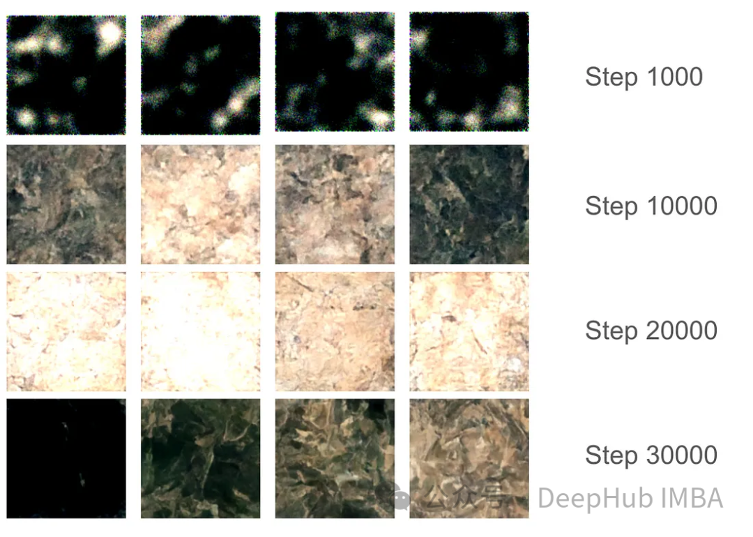
对于训练部分,我们设置了37,000步的训练,每步16个批次。由于GPU内存分配限制,图像大小被限制为128x128。使用指数移动平均(EMA)模型权重每1000步生成样本以平滑采样,并保存模型版本。
在最初的1000步训练中,模型开始捕捉一些特征,但仍然错过了某些区域。在10000步左右,这个模型开始产生有希望的结果,进步变得更加明显。在3万步的最后,结果的质量显著提高,但仍然存在黑色图像。这只是因为模型没有足够的样本种类,真实图像的数据分布并没有完全映射到高斯分布。
有了最终的模型权重,我们可以生成一些图片。尽管由于128x128的尺寸限制,图像质量受到限制,但该模型的表现还是不错的。
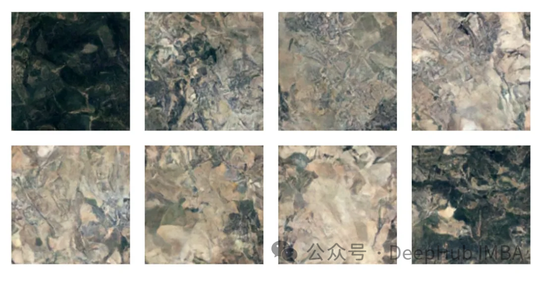
注:本文使用的数据集是森林地形的卫星图片,具体获取方式请参考源代码中的ETL部分。
总结
我们已经完整的介绍了有关扩散模型的必要知识,并且使用Pytorch进行了完整的实现,本文的代码:
https://github.com/Camaltra/this-is-not-real-aerial-imagery/
The above is the detailed content of Implementing noise removal diffusion model using PyTorch. For more information, please follow other related articles on the PHP Chinese website!

Hot AI Tools

Undresser.AI Undress
AI-powered app for creating realistic nude photos

AI Clothes Remover
Online AI tool for removing clothes from photos.

Undress AI Tool
Undress images for free

Clothoff.io
AI clothes remover

Video Face Swap
Swap faces in any video effortlessly with our completely free AI face swap tool!

Hot Article

Hot Tools

Notepad++7.3.1
Easy-to-use and free code editor

SublimeText3 Chinese version
Chinese version, very easy to use

Zend Studio 13.0.1
Powerful PHP integrated development environment

Dreamweaver CS6
Visual web development tools

SublimeText3 Mac version
God-level code editing software (SublimeText3)

Hot Topics
 1386
1386
 52
52
 iFlytek: Huawei's Ascend 910B's capabilities are basically comparable to Nvidia's A100, and they are working together to create a new base for my country's general artificial intelligence
Oct 22, 2023 pm 06:13 PM
This site reported on October 22 that in the third quarter of this year, iFlytek achieved a net profit of 25.79 million yuan, a year-on-year decrease of 81.86%; the net profit in the first three quarters was 99.36 million yuan, a year-on-year decrease of 76.36%. Jiang Tao, Vice President of iFlytek, revealed at the Q3 performance briefing that iFlytek has launched a special research project with Huawei Shengteng in early 2023, and jointly developed a high-performance operator library with Huawei to jointly create a new base for China's general artificial intelligence, allowing domestic large-scale models to be used. The architecture is based on independently innovative software and hardware. He pointed out that the current capabilities of Huawei’s Ascend 910B are basically comparable to Nvidia’s A100. At the upcoming iFlytek 1024 Global Developer Festival, iFlytek and Huawei will make further joint announcements on the artificial intelligence computing power base. He also mentioned,
 The perfect combination of PyCharm and PyTorch: detailed installation and configuration steps
Feb 21, 2024 pm 12:00 PM
PyCharm is a powerful integrated development environment (IDE), and PyTorch is a popular open source framework in the field of deep learning. In the field of machine learning and deep learning, using PyCharm and PyTorch for development can greatly improve development efficiency and code quality. This article will introduce in detail how to install and configure PyTorch in PyCharm, and attach specific code examples to help readers better utilize the powerful functions of these two. Step 1: Install PyCharm and Python
 Introduction to five sampling methods in natural language generation tasks and Pytorch code implementation
Feb 20, 2024 am 08:50 AM
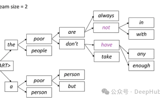
In natural language generation tasks, sampling method is a technique to obtain text output from a generative model. This article will discuss 5 common methods and implement them using PyTorch. 1. GreedyDecoding In greedy decoding, the generative model predicts the words of the output sequence based on the input sequence time step by time. At each time step, the model calculates the conditional probability distribution of each word, and then selects the word with the highest conditional probability as the output of the current time step. This word becomes the input to the next time step, and the generation process continues until some termination condition is met, such as a sequence of a specified length or a special end marker. The characteristic of GreedyDecoding is that each time the current conditional probability is the best
 Implementing noise removal diffusion model using PyTorch
Jan 14, 2024 pm 10:33 PM
Before we understand the working principle of the Denoising Diffusion Probabilistic Model (DDPM) in detail, let us first understand some of the development of generative artificial intelligence, which is also one of the basic research of DDPM. VAEVAE uses an encoder, a probabilistic latent space, and a decoder. During training, the encoder predicts the mean and variance of each image and samples these values from a Gaussian distribution. The result of the sampling is passed to the decoder, which converts the input image into a form similar to the output image. KL divergence is used to calculate the loss. A significant advantage of VAE is its ability to generate diverse images. In the sampling stage, one can directly sample from the Gaussian distribution and generate new images through the decoder. GAN has made great progress in variational autoencoders (VAEs) in just one year.
 Tutorial on installing PyCharm with PyTorch
Feb 24, 2024 am 10:09 AM
As a powerful deep learning framework, PyTorch is widely used in various machine learning projects. As a powerful Python integrated development environment, PyCharm can also provide good support when implementing deep learning tasks. This article will introduce in detail how to install PyTorch in PyCharm and provide specific code examples to help readers quickly get started using PyTorch for deep learning tasks. Step 1: Install PyCharm First, we need to make sure we have
 Deep Learning with PHP and PyTorch
Jun 19, 2023 pm 02:43 PM
Deep learning is an important branch in the field of artificial intelligence and has received more and more attention in recent years. In order to be able to conduct deep learning research and applications, it is often necessary to use some deep learning frameworks to help achieve it. In this article, we will introduce how to use PHP and PyTorch for deep learning. 1. What is PyTorch? PyTorch is an open source machine learning framework developed by Facebook. It can help us quickly create and train deep learning models. PyTorc
 so fast! Recognize video speech into text in just a few minutes with less than 10 lines of code
Feb 27, 2024 pm 01:55 PM
Hello everyone, I am Kite. Two years ago, the need to convert audio and video files into text content was difficult to achieve, but now it can be easily solved in just a few minutes. It is said that in order to obtain training data, some companies have fully crawled videos on short video platforms such as Douyin and Kuaishou, and then extracted the audio from the videos and converted them into text form to be used as training corpus for big data models. If you need to convert a video or audio file to text, you can try this open source solution available today. For example, you can search for the specific time points when dialogues in film and television programs appear. Without further ado, let’s get to the point. Whisper is OpenAI’s open source Whisper. Of course it is written in Python. It only requires a few simple installation packages.
 How to install pytorch in pycharm
Dec 08, 2023 pm 03:05 PM
Installation steps: 1. Open PyCharm and create a new Python project; 2. In the bottom status bar of PyCharm, click the "Terminal" icon to open the terminal window; 3. In the terminal window, use the pip command to install PyTorch, according to the system and requirements, you can choose different installation methods; 4. After the installation is completed, you can write code in PyCharm and import the PyTorch library to use it.


