Excel tip: How to use ranking to identify values ​​in another column

first aid! How to mark the ranking of one column in another column based on the number in excel

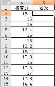
1. Select the first cell under "Ranking", as shown in the figure:

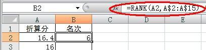
2. Enter "=RANK(A2,A$2:A$15)" where you enter the formula, press Enter after entering, and the ranking will be displayed in the cell.

means using the RANK function to feedback the sorting situation. The syntax of the RANK function is: RANK (Number, ref, order), Number is the source data cell, ref is the comparison data range, and order is a reference value (if not If you write "0", it means sorting in descending order, that is, from high to low. If you write "1", it means sorting in ascending order).

So the meaning of this formula is to use the data value of A2 to compare all the values ​​in the area from A2 to A15 in descending order and then output the sorted value.

PS. You can change the value of the corresponding ref part according to your actual situation. Be careful not to delete the $ sign.

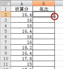
3. Continue to select cell B2, place the mouse on the small black square in the lower right corner, click and hold the left button, and drag down all the cells to be filled with rankings.

What is the formula for automatically generating rankings in a spreadsheet

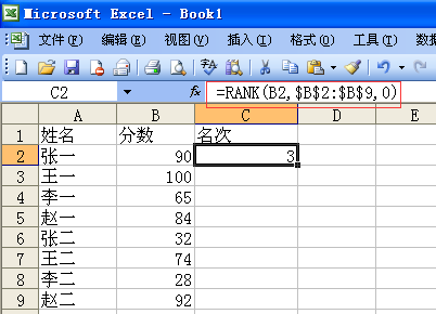
The formula for automatically generating rankings in a spreadsheet can use the function RANK. The usage is: =RANK(number, ref, order). number is the number that needs to be ranked; ref is the data source; ordef is the number. If it is 0, it means sorting in descending order, and if it is not 0, it means sorting in ascending order. The following examples illustrate how to apply. As shown below, in column C, personal rankings are listed from high to low according to scores:

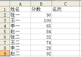
1. Enter the formula in cell C2: =RANK(B2,$B$2:$B$9,0), press Enter, and Zhang Yi’s ranking will be automatically calculated;

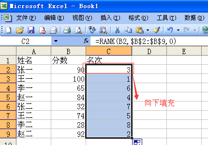
2. Click cell C2, move the cursor to the lower right corner of the cell, and hold down the mouse to fill down to cell C9.

illustrate:

1. When sorting in descending order, the last 0 in the formula does not need to be entered, that is, =RANK(B2,$B$2:$B$9);

2. When sorting in ascending order, the third value in the formula needs to enter any number that is not equal to 0;

3. To ensure that the referenced data source is accurate and unchanged, the absolute reference symbol "$" should be added in front of the referenced data cell.

How to use excel to rank student performance

Method/Step

Step one: Find the EXCEL table and double-click to enter

Step 2: Edit the student’s information, including the student’s student number, name, grades in each subject, etc.

Step 3: Enter: average score in cell I2 on the right side of sports, and calculate below. After getting Gao Lulu's average score, " " is displayed in the lower right corner of cell I2, and directly drag it back with the mouse until I9.

Step 4: Set the number of decimal points for the average score. Select the entire column I, right-click, select Format Cells, in the second: Value, change the 2 decimal places on the right to 0, OK.

Step 5: Select row 1 A1-I1, click on the data above, select filter, auto-filter, and OK.

Step 6: Select the button behind the average score and select the top descending order,

7

Step 7: Enter the ranking after the average score, and rank according to the average score. The ranking after 89 is 1, the ranking after 88 is 2, and so on

How to do excel score ranking

How to do excel score ranking?

01. In this example, students are ranked based on their scores in column C, and the ranking results are displayed in column D.

02. Select cell D2, enter [=] in the cell, and then click the [Insert Function] button.

03. The [Insert Function] dialog box pops up:

Select the [All] option in [or select a category];

Select the [RANK] function in [Select Function], and then click the [OK] button.

04. The [Function Parameters] dialog box pops up:

Move the cursor into the dialog box behind the first parameter and directly select cell C2 in the table;

Move the cursor into the dialog box behind the second parameter, select the C2:C11 cell range, and then press the F4 key for absolute reference. After setting all parameters, click the [OK] button.

05. Return to the worksheet, you can see that cell C2 ranks ninth among all results.

Select cell D2, click the left mouse button and drag the mouse to rank the remaining results.

06. Select any cell in the table and click the [Data]-[Sort] button in sequence.

07. The [Sort] dialog box pops up:

Select the [Ranking] option in [Main Keywords];

Select [Value] in [Sort by];

Select the [Ascending Order] option in [Order], and then click the [OK] button.

08. Return to the worksheet, and the arrangement of column D changes to ascending order from [1] to [10].



The above is the detailed content of Excel tip: How to use ranking to identify values ​​in another column. For more information, please follow other related articles on the PHP Chinese website!