

Theory and techniques of weight update in neural networks


Weight update in neural network is to adjust the connection weights between neurons in the network through methods such as back propagation algorithm to improve the performance of the network. This article will introduce the concept and method of weight update to help readers better understand the training process of neural networks.
1. Concept
The weights in neural networks are parameters connecting different neurons and determine the strength of signal transmission. Each neuron receives the signal from the previous layer, multiplies it by the weight of the connection, adds a bias term, and is finally activated through the activation function and passed to the next layer. Therefore, the size of the weight directly affects the strength and direction of the signal, which in turn affects the output of the neural network.
The purpose of weight update is to optimize the performance of the neural network. During the training process, the neural network adapts to the training data by continuously adjusting the weights between neurons to improve the prediction ability on the test data. By adjusting the weights, the neural network can better fit the training data, thereby improving the prediction accuracy. In this way, the neural network can more accurately predict the results of unknown data and achieve better performance.
2. Method
Commonly used weight update methods in neural networks include gradient descent, stochastic gradient descent, and batch gradient descent.
Gradient descent method
The gradient descent method is one of the most basic weight update methods. Its basic idea is to calculate the loss function to update the weight. The gradient (that is, the derivative of the loss function with respect to the weight) is used to update the weight to minimize the loss function. Specifically, the steps of the gradient descent method are as follows:
First, we need to define a loss function to measure the performance of the neural network on the training data. Usually, we will choose the mean square error (MSE) as the loss function, which is defined as follows:
MSE=\frac{1}{n}\sum_{i=1} ^{n}(y_i-\hat{y_i})^2
Where, y_i represents the true value of the i-th sample, \hat{y_i} represents the neural network's response to the i-th sample The predicted value of samples, n represents the total number of samples.
Then, we need to calculate the derivative of the loss function with respect to the weight, that is, the gradient. Specifically, for each weight w_{ij} in the neural network, its gradient can be calculated by the following formula:
\frac{\partial MSE}{\partial w_{ij }}=\frac{2}{n}\sum_{k=1}^{n}(y_k-\hat{y_k})\cdot f'(\sum_{j=1}^{m}w_{ij }x_{kj})\cdot x_{ki}
Among them, n represents the total number of samples, m represents the input layer size of the neural network, and x_{kj} represents the kth sample For the jth input feature, f(\cdot) represents the activation function, and f'(\cdot) represents the derivative of the activation function.
Finally, we can update the weights through the following formula:
w_{ij}=w_{ij}-\alpha\cdot\ frac{\partial MSE}{\partial w_{ij}}
Among them, \alpha represents the learning rate, which controls the step size of weight update.
Stochastic gradient descent method
The stochastic gradient descent method is a variant of the gradient descent method. Its basic idea is to randomly select each time A sample is used to calculate the gradient and update the weights. Compared to the gradient descent method, the stochastic gradient descent method can converge faster and be more efficient when processing large-scale data sets. Specifically, the steps of the stochastic gradient descent method are as follows:
First, we need to shuffle the training data and randomly select a sample x_k to calculate the gradient. We can then calculate the derivative of the loss function with respect to the weights via the following formula:
\frac{\partial MSE}{\partial w_{ij}}=2(y_k-\hat {y_k})\cdot f'(\sum_{j=1}^{m}w_{ij}x_{kj})\cdot x_{ki}
where, y_k represents the true value of the k-th sample, \hat{y_k} represents the predicted value of the k-th sample by the neural network.
Finally, we can update the weights through the following formula:
w_{ij}=w_{ij}-\alpha\cdot\ frac{\partial MSE}{\partial w_{ij}}
Among them, \alpha represents the learning rate, which controls the step size of weight update.
Batch gradient descent method
The batch gradient descent method is another variant of the gradient descent method. The basic idea is to use A mini-batch of samples is used to calculate the gradient and update the weights. Compared with gradient descent and stochastic gradient descent, batch gradient descent can converge more stably and is more efficient when processing small-scale data sets. Specifically, the steps of the batch gradient descent method are as follows:
First, we need to divide the training data into several mini-batches of equal size, each mini-batch contains b samples. We can then calculate the average gradient of the loss function against the weights on each mini-batch, which is:
\frac{1}{b}\sum_{k=1}^{ b}\frac{\partial MSE}{\partial w_{ij}}
where b represents the mini-batch size. Finally, we can update the weights through the following formula:
w_{ij}=w_{ij}-\alpha\cdot\frac{1}{b}\sum_{k= 1}^{b}\frac{\partial MSE}{\partial w_{ij}}
Among them, \alpha represents the learning rate, which controls the step size of weight update.
The above is the detailed content of Theory and techniques of weight update in neural networks. For more information, please follow other related articles on the PHP Chinese website!

Hot AI Tools

Undresser.AI Undress
AI-powered app for creating realistic nude photos

AI Clothes Remover
Online AI tool for removing clothes from photos.

Undress AI Tool
Undress images for free

Clothoff.io
AI clothes remover

Video Face Swap
Swap faces in any video effortlessly with our completely free AI face swap tool!

Hot Article
Hot Tools

Notepad++7.3.1
Easy-to-use and free code editor

SublimeText3 Chinese version
Chinese version, very easy to use

Zend Studio 13.0.1
Powerful PHP integrated development environment

Dreamweaver CS6
Visual web development tools

SublimeText3 Mac version
God-level code editing software (SublimeText3)
Hot Topics
 1387
1387
 52
52

 Explore the concepts, differences, advantages and disadvantages of RNN, LSTM and GRU
Jan 22, 2024 pm 07:51 PM
Explore the concepts, differences, advantages and disadvantages of RNN, LSTM and GRU
Jan 22, 2024 pm 07:51 PM
In time series data, there are dependencies between observations, so they are not independent of each other. However, traditional neural networks treat each observation as independent, which limits the model's ability to model time series data. To solve this problem, Recurrent Neural Network (RNN) was introduced, which introduced the concept of memory to capture the dynamic characteristics of time series data by establishing dependencies between data points in the network. Through recurrent connections, RNN can pass previous information into the current observation to better predict future values. This makes RNN a powerful tool for tasks involving time series data. But how does RNN achieve this kind of memory? RNN realizes memory through the feedback loop in the neural network. This is the difference between RNN and traditional neural network.
 A case study of using bidirectional LSTM model for text classification
Jan 24, 2024 am 10:36 AM
A case study of using bidirectional LSTM model for text classification
Jan 24, 2024 am 10:36 AM
The bidirectional LSTM model is a neural network used for text classification. Below is a simple example demonstrating how to use bidirectional LSTM for text classification tasks. First, we need to import the required libraries and modules: importosimportnumpyasnpfromkeras.preprocessing.textimportTokenizerfromkeras.preprocessing.sequenceimportpad_sequencesfromkeras.modelsimportSequentialfromkeras.layersimportDense,Em
 Calculating floating point operands (FLOPS) for neural networks
Jan 22, 2024 pm 07:21 PM
Calculating floating point operands (FLOPS) for neural networks
Jan 22, 2024 pm 07:21 PM
FLOPS is one of the standards for computer performance evaluation, used to measure the number of floating point operations per second. In neural networks, FLOPS is often used to evaluate the computational complexity of the model and the utilization of computing resources. It is an important indicator used to measure the computing power and efficiency of a computer. A neural network is a complex model composed of multiple layers of neurons used for tasks such as data classification, regression, and clustering. Training and inference of neural networks requires a large number of matrix multiplications, convolutions and other calculation operations, so the computational complexity is very high. FLOPS (FloatingPointOperationsperSecond) can be used to measure the computational complexity of neural networks to evaluate the computational resource usage efficiency of the model. FLOP
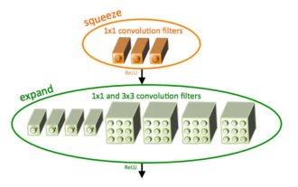 Introduction to SqueezeNet and its characteristics
Jan 22, 2024 pm 07:15 PM
Introduction to SqueezeNet and its characteristics
Jan 22, 2024 pm 07:15 PM
SqueezeNet is a small and precise algorithm that strikes a good balance between high accuracy and low complexity, making it ideal for mobile and embedded systems with limited resources. In 2016, researchers from DeepScale, University of California, Berkeley, and Stanford University proposed SqueezeNet, a compact and efficient convolutional neural network (CNN). In recent years, researchers have made several improvements to SqueezeNet, including SqueezeNetv1.1 and SqueezeNetv2.0. Improvements in both versions not only increase accuracy but also reduce computational costs. Accuracy of SqueezeNetv1.1 on ImageNet dataset
 Definition and structural analysis of fuzzy neural network
Jan 22, 2024 pm 09:09 PM
Definition and structural analysis of fuzzy neural network
Jan 22, 2024 pm 09:09 PM
Fuzzy neural network is a hybrid model that combines fuzzy logic and neural networks to solve fuzzy or uncertain problems that are difficult to handle with traditional neural networks. Its design is inspired by the fuzziness and uncertainty in human cognition, so it is widely used in control systems, pattern recognition, data mining and other fields. The basic architecture of fuzzy neural network consists of fuzzy subsystem and neural subsystem. The fuzzy subsystem uses fuzzy logic to process input data and convert it into fuzzy sets to express the fuzziness and uncertainty of the input data. The neural subsystem uses neural networks to process fuzzy sets for tasks such as classification, regression or clustering. The interaction between the fuzzy subsystem and the neural subsystem makes the fuzzy neural network have more powerful processing capabilities and can
 Image denoising using convolutional neural networks
Jan 23, 2024 pm 11:48 PM
Image denoising using convolutional neural networks
Jan 23, 2024 pm 11:48 PM
Convolutional neural networks perform well in image denoising tasks. It utilizes the learned filters to filter the noise and thereby restore the original image. This article introduces in detail the image denoising method based on convolutional neural network. 1. Overview of Convolutional Neural Network Convolutional neural network is a deep learning algorithm that uses a combination of multiple convolutional layers, pooling layers and fully connected layers to learn and classify image features. In the convolutional layer, the local features of the image are extracted through convolution operations, thereby capturing the spatial correlation in the image. The pooling layer reduces the amount of calculation by reducing the feature dimension and retains the main features. The fully connected layer is responsible for mapping learned features and labels to implement image classification or other tasks. The design of this network structure makes convolutional neural networks useful in image processing and recognition.
 Compare the similarities, differences and relationships between dilated convolution and atrous convolution
Jan 22, 2024 pm 10:27 PM
Compare the similarities, differences and relationships between dilated convolution and atrous convolution
Jan 22, 2024 pm 10:27 PM
Dilated convolution and dilated convolution are commonly used operations in convolutional neural networks. This article will introduce their differences and relationships in detail. 1. Dilated convolution Dilated convolution, also known as dilated convolution or dilated convolution, is an operation in a convolutional neural network. It is an extension based on the traditional convolution operation and increases the receptive field of the convolution kernel by inserting holes in the convolution kernel. This way, the network can better capture a wider range of features. Dilated convolution is widely used in the field of image processing and can improve the performance of the network without increasing the number of parameters and the amount of calculation. By expanding the receptive field of the convolution kernel, dilated convolution can better process the global information in the image, thereby improving the effect of feature extraction. The main idea of dilated convolution is to introduce some
 Steps to write a simple neural network using Rust
Jan 23, 2024 am 10:45 AM
Steps to write a simple neural network using Rust
Jan 23, 2024 am 10:45 AM
Rust is a systems-level programming language focused on safety, performance, and concurrency. It aims to provide a safe and reliable programming language suitable for scenarios such as operating systems, network applications, and embedded systems. Rust's security comes primarily from two aspects: the ownership system and the borrow checker. The ownership system enables the compiler to check code for memory errors at compile time, thus avoiding common memory safety issues. By forcing checking of variable ownership transfers at compile time, Rust ensures that memory resources are properly managed and released. The borrow checker analyzes the life cycle of the variable to ensure that the same variable will not be accessed by multiple threads at the same time, thereby avoiding common concurrency security issues. By combining these two mechanisms, Rust is able to provide
