

Application of Diffusion Model in Analytical Image Processing


In the field of machine learning, diffusion models play a wide role in image processing. It is used in multiple image processing tasks, including image denoising, image enhancement, and image segmentation. The main advantage of the diffusion model is that it can effectively handle noise in images, while also enhancing image details and contrast, and enabling accurate image segmentation. In addition, diffusion models are highly computationally efficient and easy to implement. In summary, diffusion models play an important role in image processing, providing us with a powerful tool to improve image quality and extract image features.
The role of diffusion model in image processing
The diffusion model is a machine learning model based on partial differential equations, mainly used in images processing areas. Its basic principle is to simulate the physical diffusion process and achieve image denoising, enhancement, segmentation and other processing operations by controlling the parameters of partial differential equations. This model was first proposed by Perona and Malik in 1990. Its core idea is to gradually smooth or diffuse the information in the image by adjusting the parameters of the partial differential equation. Specifically, the diffusion model compares the difference between a pixel in the image and its neighbor pixels and adjusts the intensity value of the pixel based on the size of the difference. Doing so reduces noise in the image and enhances image detail. Diffusion models are widely used in image processing. For example, in terms of image denoising, it can effectively remove noise in images and make them clearer. In terms of image enhancement, it can enhance the contrast and details of the image, making the image more vivid. In image segmentation
Specifically, the role of the diffusion model in image processing is as follows:
1. Image denoising
The diffusion model can simulate the diffusion process of noise and gradually smooth the noise to achieve image denoising. Specifically, the diffusion model can use partial differential equations to describe the diffusion process of noise in the image, and smooth the noise by repeatedly iteratively solving the differential equations. This method can effectively remove common image noise such as Gaussian noise and salt-and-pepper noise.
2. Image enhancement
The diffusion model can achieve image enhancement by increasing the details and contrast of the image. Specifically, the diffusion model can use partial differential equations to describe the diffusion process of color or intensity in an image, and increase the detail and contrast of the image by controlling parameters such as diffusion coefficient and time step. This method can effectively enhance the texture, edges and other details of the image, making the image clearer and more vivid.
3. Image segmentation
The diffusion model can achieve image segmentation by simulating the diffusion process of edges. Specifically, the diffusion model can use partial differential equations to describe the diffusion process of gray values in the image, and achieve image segmentation by controlling parameters such as diffusion coefficient and time step. This method can effectively segment different objects or areas in the image, providing a basis for subsequent image analysis and processing.
Why the diffusion model can generate details when generating images
The diffusion model uses partial differential equations to describe the distribution of color or intensity in space and time. Evolution, by repeatedly iteratively solving the differential equation, the final state of the image is obtained. The reasons why the diffusion model can generate details are as follows:
1. Simulate the physical process
The basic principle of the diffusion model is to simulate the physical process , that is, the diffusion of color or intensity. In this process, the value of each pixel is affected by the pixels around it, so each pixel is updated multiple times when the differential equation is iteratively solved. This iterative process repeatedly strengthens the interaction between pixels, resulting in more detailed images.
2. Control parameters
There are many control parameters in the diffusion model, such as diffusion coefficient, time step, etc. These parameters can affect the image generation process. By adjusting these parameters, you can control the direction and level of detail in the image. For example, increasing the diffusion coefficient can cause colors or intensities to diffuse faster, resulting in a blurrier image; decreasing the time step can increase the number of iterations, resulting in a more detailed image.
3. Randomness
There are also some random factors in the diffusion model, such as initial values, noise, etc., which can increase Image variation and detail. For example, adding some noise to the initial value can make the image generation process more random, thereby generating a more detailed image; during the iterative process, you can also add some random perturbations to increase the changes and details of the image.
4. Multi-scale processing
The diffusion model can increase the details of the image through multi-scale processing. Specifically, the original image can be downsampled first to generate a smaller image, and then the diffusion model can be solved on this smaller image. The advantage of this is that it can make the details of the image more prominent and also improve the computational efficiency of the model.
5. Combine with other models
Diffusion models can be used in conjunction with other models to further increase image detail. For example, the diffusion model can be used in combination with a generative adversarial network (GAN), using the image generated by the GAN as the initial image of the diffusion model, and then further adding details through the diffusion model to generate a more realistic image.
The mathematical basis of the diffusion model
The mathematical basis of the diffusion model is the partial differential equation, its basic form is:
∂u/∂t=div(c(∇u)), where u(x,y,t) represents the image gray value at the position (x,y) at time t, c( ∇u) represents the diffusion coefficient, div represents the divergence operator, and ∇ represents the gradient operator.
This equation describes the diffusion process of gray value in a grayscale image, where c(∇u) controls the direction and speed of diffusion. Usually, c(∇u) is a nonlinear function, which can be adjusted according to the characteristics of the image to achieve different image processing effects. For example, when c(∇u) is a Gaussian function, the diffusion model can be used to remove Gaussian noise; when c(∇u) is a gradient function, the diffusion model can be used to enhance the edge features of the image.
The solution process of the diffusion model usually adopts an iterative method, that is, in each step, the gray value of the image is updated by solving the partial differential equation. For 2D images, the diffusion model can be iterated in both x and y directions. During the iteration process, parameters such as diffusion coefficient and time step can also be adjusted to achieve different image processing effects.
The reason why the loss of the diffusion model decreases very quickly
In the diffusion model, the loss function often decreases very quickly. This is due to Due to the characteristics of the diffusion model itself.
In machine learning, the application of the diffusion model is mainly to perform denoising or edge detection on images. These treatments can usually be transformed into an optimization problem of solving a partial differential equation, that is, minimizing a loss function.
In diffusion models, the loss function is usually defined as the difference between the original image and the processed image. Therefore, the process of optimizing the loss function is to adjust the model parameters to make the processed image as close as possible to the original image. Since the mathematical expression of the diffusion model is relatively simple and its model parameters are usually small, the loss function tends to decrease very quickly during the training process.
In addition, the loss function of the diffusion model is usually a convex function, which means that during the training process, the decline speed of the loss function will not have obvious oscillations, but will appear smooth. downward trend. This is also one of the reasons why the loss function decreases quickly.
In addition to the above reasons, the rapid decline of the loss function of the diffusion model is also related to its model structure and optimization algorithm. Diffusion models usually use implicit numerical methods to solve partial differential equations. This method has high computational efficiency and numerical stability, and can effectively solve numerical errors and time-consuming problems in the numerical solution process. In addition, the optimization algorithm of the diffusion model usually uses optimization algorithms such as gradient descent. These algorithms can effectively reduce the computational complexity when processing high-dimensional data, thereby speeding up the decline of the loss function.
The rapid decline of the loss function of the diffusion model is also related to the nature of the model and parameter selection. In diffusion models, the parameters of the model are usually set as constants or time-related functions. The choice of these parameters can affect the performance of the model and the rate of decline of the loss function. Generally speaking, setting appropriate parameters can speed up model training and improve model performance.
In addition, in the diffusion model, there are some optimization techniques that can further speed up the decline of the loss function. For example, an optimization algorithm using adaptive step size can automatically adjust the update step size of model parameters according to changes in the loss function, thereby speeding up the convergence of the model. In addition, using techniques such as batch normalization and residual connection can also effectively improve the training speed and performance of the model.
Diffusion model and neural network
In machine learning, diffusion model is mainly used in the fields of image processing and computer vision. For example, the diffusion model can be used to perform image denoising or edge detection. In addition, the diffusion model can also be used in image segmentation, target recognition and other fields. The advantage of the diffusion model is that it can handle high-dimensional data and has strong noise immunity and smoothness, but its computational efficiency is low and it requires a lot of computing resources and time.
Neural networks are widely used in machine learning and can be used in image recognition, natural language processing, speech recognition and other fields. Compared with diffusion models, neural networks have stronger expression and generalization capabilities, can handle various types of data, and can automatically learn features. However, the neural network has a large number of parameters and requires a large amount of data and computing resources for training. At the same time, its model structure is relatively complex and requires certain technology and experience to design and optimize.
In practical applications, diffusion models and neural networks are often used in combination to give full play to their respective advantages. For example, in image processing, you can first use the diffusion model to denoise and smooth the image, and then input the processed image into the neural network for feature extraction and classification recognition. This combination can improve the accuracy and robustness of the model, while also accelerating the model training and inference process.
The above is the detailed content of Application of Diffusion Model in Analytical Image Processing. For more information, please follow other related articles on the PHP Chinese website!

Hot AI Tools

Undresser.AI Undress
AI-powered app for creating realistic nude photos

AI Clothes Remover
Online AI tool for removing clothes from photos.

Undress AI Tool
Undress images for free

Clothoff.io
AI clothes remover

AI Hentai Generator
Generate AI Hentai for free.

Hot Article
Hot Tools

Notepad++7.3.1
Easy-to-use and free code editor

SublimeText3 Chinese version
Chinese version, very easy to use

Zend Studio 13.0.1
Powerful PHP integrated development environment

Dreamweaver CS6
Visual web development tools

SublimeText3 Mac version
God-level code editing software (SublimeText3)
Hot Topics


 This article will take you to understand SHAP: model explanation for machine learning
Jun 01, 2024 am 10:58 AM
This article will take you to understand SHAP: model explanation for machine learning
Jun 01, 2024 am 10:58 AM
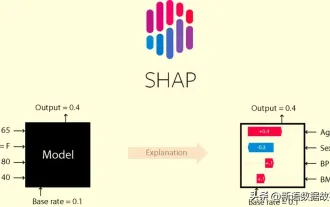
In the fields of machine learning and data science, model interpretability has always been a focus of researchers and practitioners. With the widespread application of complex models such as deep learning and ensemble methods, understanding the model's decision-making process has become particularly important. Explainable AI|XAI helps build trust and confidence in machine learning models by increasing the transparency of the model. Improving model transparency can be achieved through methods such as the widespread use of multiple complex models, as well as the decision-making processes used to explain the models. These methods include feature importance analysis, model prediction interval estimation, local interpretability algorithms, etc. Feature importance analysis can explain the decision-making process of a model by evaluating the degree of influence of the model on the input features. Model prediction interval estimate
 Transparent! An in-depth analysis of the principles of major machine learning models!
Apr 12, 2024 pm 05:55 PM
Transparent! An in-depth analysis of the principles of major machine learning models!
Apr 12, 2024 pm 05:55 PM
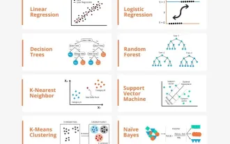
In layman’s terms, a machine learning model is a mathematical function that maps input data to a predicted output. More specifically, a machine learning model is a mathematical function that adjusts model parameters by learning from training data to minimize the error between the predicted output and the true label. There are many models in machine learning, such as logistic regression models, decision tree models, support vector machine models, etc. Each model has its applicable data types and problem types. At the same time, there are many commonalities between different models, or there is a hidden path for model evolution. Taking the connectionist perceptron as an example, by increasing the number of hidden layers of the perceptron, we can transform it into a deep neural network. If a kernel function is added to the perceptron, it can be converted into an SVM. this one
 Identify overfitting and underfitting through learning curves
Apr 29, 2024 pm 06:50 PM
Identify overfitting and underfitting through learning curves
Apr 29, 2024 pm 06:50 PM
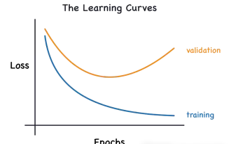
This article will introduce how to effectively identify overfitting and underfitting in machine learning models through learning curves. Underfitting and overfitting 1. Overfitting If a model is overtrained on the data so that it learns noise from it, then the model is said to be overfitting. An overfitted model learns every example so perfectly that it will misclassify an unseen/new example. For an overfitted model, we will get a perfect/near-perfect training set score and a terrible validation set/test score. Slightly modified: "Cause of overfitting: Use a complex model to solve a simple problem and extract noise from the data. Because a small data set as a training set may not represent the correct representation of all data." 2. Underfitting Heru
 The evolution of artificial intelligence in space exploration and human settlement engineering
Apr 29, 2024 pm 03:25 PM
The evolution of artificial intelligence in space exploration and human settlement engineering
Apr 29, 2024 pm 03:25 PM
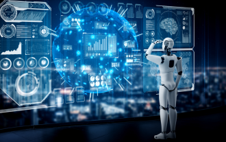
In the 1950s, artificial intelligence (AI) was born. That's when researchers discovered that machines could perform human-like tasks, such as thinking. Later, in the 1960s, the U.S. Department of Defense funded artificial intelligence and established laboratories for further development. Researchers are finding applications for artificial intelligence in many areas, such as space exploration and survival in extreme environments. Space exploration is the study of the universe, which covers the entire universe beyond the earth. Space is classified as an extreme environment because its conditions are different from those on Earth. To survive in space, many factors must be considered and precautions must be taken. Scientists and researchers believe that exploring space and understanding the current state of everything can help understand how the universe works and prepare for potential environmental crises
 Implementing Machine Learning Algorithms in C++: Common Challenges and Solutions
Jun 03, 2024 pm 01:25 PM
Implementing Machine Learning Algorithms in C++: Common Challenges and Solutions
Jun 03, 2024 pm 01:25 PM
Common challenges faced by machine learning algorithms in C++ include memory management, multi-threading, performance optimization, and maintainability. Solutions include using smart pointers, modern threading libraries, SIMD instructions and third-party libraries, as well as following coding style guidelines and using automation tools. Practical cases show how to use the Eigen library to implement linear regression algorithms, effectively manage memory and use high-performance matrix operations.
 Explainable AI: Explaining complex AI/ML models
Jun 03, 2024 pm 10:08 PM
Explainable AI: Explaining complex AI/ML models
Jun 03, 2024 pm 10:08 PM
Translator | Reviewed by Li Rui | Chonglou Artificial intelligence (AI) and machine learning (ML) models are becoming increasingly complex today, and the output produced by these models is a black box – unable to be explained to stakeholders. Explainable AI (XAI) aims to solve this problem by enabling stakeholders to understand how these models work, ensuring they understand how these models actually make decisions, and ensuring transparency in AI systems, Trust and accountability to address this issue. This article explores various explainable artificial intelligence (XAI) techniques to illustrate their underlying principles. Several reasons why explainable AI is crucial Trust and transparency: For AI systems to be widely accepted and trusted, users need to understand how decisions are made
 Outlook on future trends of Golang technology in machine learning
May 08, 2024 am 10:15 AM
Outlook on future trends of Golang technology in machine learning
May 08, 2024 am 10:15 AM
The application potential of Go language in the field of machine learning is huge. Its advantages are: Concurrency: It supports parallel programming and is suitable for computationally intensive operations in machine learning tasks. Efficiency: The garbage collector and language features ensure that the code is efficient, even when processing large data sets. Ease of use: The syntax is concise, making it easy to learn and write machine learning applications.
 Is Flash Attention stable? Meta and Harvard found that their model weight deviations fluctuated by orders of magnitude
May 30, 2024 pm 01:24 PM
Is Flash Attention stable? Meta and Harvard found that their model weight deviations fluctuated by orders of magnitude
May 30, 2024 pm 01:24 PM
MetaFAIR teamed up with Harvard to provide a new research framework for optimizing the data bias generated when large-scale machine learning is performed. It is known that the training of large language models often takes months and uses hundreds or even thousands of GPUs. Taking the LLaMA270B model as an example, its training requires a total of 1,720,320 GPU hours. Training large models presents unique systemic challenges due to the scale and complexity of these workloads. Recently, many institutions have reported instability in the training process when training SOTA generative AI models. They usually appear in the form of loss spikes. For example, Google's PaLM model experienced up to 20 loss spikes during the training process. Numerical bias is the root cause of this training inaccuracy,
