

How to build a neural network using TensorFlow


TensorFlow is a popular machine learning framework used for training and deploying various neural networks. This article discusses how to use TensorFlow to build a simple neural network and provides sample code to get you started.
The first step in building a neural network is to define the structure of the network. In TensorFlow, we can use the tf.keras module to define the layers of a neural network. The following code example defines a fully connected feed-forward neural network with two hidden layers and an output layer: ```python import tensorflow astf model = tf.keras.models.Sequential([ tf.keras.layers.Dense(units=64, activation='relu', input_shape=(input_dim,)), tf.keras.layers.Dense(units=32, activation='relu'), tf.keras.layers.Dense(units=output_dim, activation='softmax') ]) ``` In the above code, we use the `Sequential` model to build the neural network. The `Dense` layer represents a fully connected layer, specifying the number of neurons (units) and activation function (activation) of each layer. The input shape of the first hidden layer is given by `input_shape
import tensorflow as tf

model = tf.keras.Sequential([
    tf.keras.layers.Dense(64, activation='relu', input_shape=(784,)),
    tf.keras.layers.Dense(64, activation='relu'),
    tf.keras.layers.Dense(10, activation='softmax')
])In this example, we use the Sequential model to define our neural network. It is a simple stacking model where each layer builds on the previous one. We define three layers, the first and second layers are both fully connected layers with 64 neurons, and they use the ReLU activation function. The shape of the input layer is (784,) because we will be using the MNIST handwritten digits dataset, and each image in this dataset is 28x28 pixels, which expands to 784 pixels. The last layer is a fully connected layer with 10 neurons that uses a softmax activation function and is used for classification tasks such as digit classification in the MNIST dataset.
We need to compile the model and specify the optimizer, loss function and evaluation metrics. Here is an example:
model.compile(optimizer='adam',
              loss='categorical_crossentropy',
metrics=['accuracy'])In this example, we use the Adam optimizer to train our model using cross-entropy as the loss function for a multi-class classification problem. We also specified accuracy as an evaluation metric to track the model's performance during training and evaluation.
Now that we have defined the structure and training configuration of the model, we can read the data and start training the model. We will use the MNIST handwritten digits dataset as an example. The following is a code example:
from tensorflow.keras.datasets import mnist

(train_images, train_labels), (test_images, test_labels) = mnist.load_data()

train_images = train_images.reshape((60000, 784))
train_images = train_images.astype('float32') / 255

test_images = test_images.reshape((10000, 784))
test_images = test_images.astype('float32') / 255

train_labels = tf.keras.utils.to_categorical(train_labels)
test_labels = tf.keras.utils.to_categorical(test_labels)

model.fit(train_images, train_labels, epochs=5, batch_size=64)
In this example, we use the mnist.load_data() function to load the MNIST dataset. We then flattened the training and test images to 784 pixels and scaled the pixel values to be between 0 and 1. We also one-hot encode the labels in order to convert them into a classification task. Finally, we use the fit function to train our model, using training images and labels, specifying training for 5 epochs, using 64 samples for each epoch.
After training is complete, we can use the evaluate function to evaluate the performance of the model on the test set:
test_loss, test_acc = model.evaluate(test_images, test_labels)
print('Test accuracy:', test_acc)
In this example, we call evaluate with the test image and label function and print the results to show the accuracy of the model on the test set.
This is a simple example of how to build and train a neural network using TensorFlow. Of course, in real applications, you may need more complex network structures and more complex data sets. However, this example provides a good starting point to help you understand the basic usage of TensorFlow.
The complete code example is as follows:
import tensorflow as tf
from tensorflow.keras.datasets import mnist

# Define the model architecture
model = tf.keras.Sequential([
    tf.keras.layers.Dense(64, activation='relu', input_shape=(784,)),
    tf.keras.layers.Dense(64, activation='relu'),
    tf.keras.layers.Dense(10, activation='softmax')
])

# Compile the model
model.compile(optimizer='adam',
              loss='categorical_crossentropy',
              metrics=['accuracy'])

# Load the data
(train_images, train_labels), (test_images, test_labels) = mnist.load_data()

train_images = train_images.reshape((60000, 784))
train_images = train_images.astype('float32') / 255

test_images = test_images.reshape((10000, 784))
test_images = test_images.astype('float32') / 255

train_labels = tf.keras.utils.to_categorical(train_labels)
test_labels = tf.keras.utils.to_categorical(test_labels)

# Train the model
model.fit(train_images, train_labels, epochs=5, batch_size=64)

# Evaluate the model
test_loss, test_acc = model.evaluate(test_images, test_labels)
print('Test accuracy:', test_acc)The above is an example code for using TensorFlow to build a neural network, which defines a layer containing two hidden layers and an output layer. Fully connected feed-forward neural network, trained and tested using the MNIST handwritten digits dataset, and using the Adam optimizer and cross-entropy loss function. The final output is the accuracy on the test set.
The above is the detailed content of How to build a neural network using TensorFlow. For more information, please follow other related articles on the PHP Chinese website!

Hot AI Tools

Undresser.AI Undress
AI-powered app for creating realistic nude photos

AI Clothes Remover
Online AI tool for removing clothes from photos.

Undress AI Tool
Undress images for free

Clothoff.io
AI clothes remover

Video Face Swap
Swap faces in any video effortlessly with our completely free AI face swap tool!

Hot Article
Hot Tools

Notepad++7.3.1
Easy-to-use and free code editor

SublimeText3 Chinese version
Chinese version, very easy to use

Zend Studio 13.0.1
Powerful PHP integrated development environment

Dreamweaver CS6
Visual web development tools

SublimeText3 Mac version
God-level code editing software (SublimeText3)
Hot Topics


 Explore the concepts, differences, advantages and disadvantages of RNN, LSTM and GRU
Jan 22, 2024 pm 07:51 PM
Explore the concepts, differences, advantages and disadvantages of RNN, LSTM and GRU
Jan 22, 2024 pm 07:51 PM
In time series data, there are dependencies between observations, so they are not independent of each other. However, traditional neural networks treat each observation as independent, which limits the model's ability to model time series data. To solve this problem, Recurrent Neural Network (RNN) was introduced, which introduced the concept of memory to capture the dynamic characteristics of time series data by establishing dependencies between data points in the network. Through recurrent connections, RNN can pass previous information into the current observation to better predict future values. This makes RNN a powerful tool for tasks involving time series data. But how does RNN achieve this kind of memory? RNN realizes memory through the feedback loop in the neural network. This is the difference between RNN and traditional neural network.
 A case study of using bidirectional LSTM model for text classification
Jan 24, 2024 am 10:36 AM
A case study of using bidirectional LSTM model for text classification
Jan 24, 2024 am 10:36 AM
The bidirectional LSTM model is a neural network used for text classification. Below is a simple example demonstrating how to use bidirectional LSTM for text classification tasks. First, we need to import the required libraries and modules: importosimportnumpyasnpfromkeras.preprocessing.textimportTokenizerfromkeras.preprocessing.sequenceimportpad_sequencesfromkeras.modelsimportSequentialfromkeras.layersimportDense,Em
 Calculating floating point operands (FLOPS) for neural networks
Jan 22, 2024 pm 07:21 PM
Calculating floating point operands (FLOPS) for neural networks
Jan 22, 2024 pm 07:21 PM
FLOPS is one of the standards for computer performance evaluation, used to measure the number of floating point operations per second. In neural networks, FLOPS is often used to evaluate the computational complexity of the model and the utilization of computing resources. It is an important indicator used to measure the computing power and efficiency of a computer. A neural network is a complex model composed of multiple layers of neurons used for tasks such as data classification, regression, and clustering. Training and inference of neural networks requires a large number of matrix multiplications, convolutions and other calculation operations, so the computational complexity is very high. FLOPS (FloatingPointOperationsperSecond) can be used to measure the computational complexity of neural networks to evaluate the computational resource usage efficiency of the model. FLOP
 Introduction to SqueezeNet and its characteristics
Jan 22, 2024 pm 07:15 PM
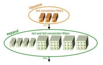
Introduction to SqueezeNet and its characteristics
Jan 22, 2024 pm 07:15 PM
SqueezeNet is a small and precise algorithm that strikes a good balance between high accuracy and low complexity, making it ideal for mobile and embedded systems with limited resources. In 2016, researchers from DeepScale, University of California, Berkeley, and Stanford University proposed SqueezeNet, a compact and efficient convolutional neural network (CNN). In recent years, researchers have made several improvements to SqueezeNet, including SqueezeNetv1.1 and SqueezeNetv2.0. Improvements in both versions not only increase accuracy but also reduce computational costs. Accuracy of SqueezeNetv1.1 on ImageNet dataset
 Definition and structural analysis of fuzzy neural network
Jan 22, 2024 pm 09:09 PM
Definition and structural analysis of fuzzy neural network
Jan 22, 2024 pm 09:09 PM
Fuzzy neural network is a hybrid model that combines fuzzy logic and neural networks to solve fuzzy or uncertain problems that are difficult to handle with traditional neural networks. Its design is inspired by the fuzziness and uncertainty in human cognition, so it is widely used in control systems, pattern recognition, data mining and other fields. The basic architecture of fuzzy neural network consists of fuzzy subsystem and neural subsystem. The fuzzy subsystem uses fuzzy logic to process input data and convert it into fuzzy sets to express the fuzziness and uncertainty of the input data. The neural subsystem uses neural networks to process fuzzy sets for tasks such as classification, regression or clustering. The interaction between the fuzzy subsystem and the neural subsystem makes the fuzzy neural network have more powerful processing capabilities and can
 Image denoising using convolutional neural networks
Jan 23, 2024 pm 11:48 PM
Image denoising using convolutional neural networks
Jan 23, 2024 pm 11:48 PM
Convolutional neural networks perform well in image denoising tasks. It utilizes the learned filters to filter the noise and thereby restore the original image. This article introduces in detail the image denoising method based on convolutional neural network. 1. Overview of Convolutional Neural Network Convolutional neural network is a deep learning algorithm that uses a combination of multiple convolutional layers, pooling layers and fully connected layers to learn and classify image features. In the convolutional layer, the local features of the image are extracted through convolution operations, thereby capturing the spatial correlation in the image. The pooling layer reduces the amount of calculation by reducing the feature dimension and retains the main features. The fully connected layer is responsible for mapping learned features and labels to implement image classification or other tasks. The design of this network structure makes convolutional neural networks useful in image processing and recognition.
 causal convolutional neural network
Jan 24, 2024 pm 12:42 PM
causal convolutional neural network
Jan 24, 2024 pm 12:42 PM
Causal convolutional neural network is a special convolutional neural network designed for causality problems in time series data. Compared with conventional convolutional neural networks, causal convolutional neural networks have unique advantages in retaining the causal relationship of time series and are widely used in the prediction and analysis of time series data. The core idea of causal convolutional neural network is to introduce causality in the convolution operation. Traditional convolutional neural networks can simultaneously perceive data before and after the current time point, but in time series prediction, this may lead to information leakage problems. Because the prediction results at the current time point will be affected by the data at future time points. The causal convolutional neural network solves this problem. It can only perceive the current time point and previous data, but cannot perceive future data.
 Compare the similarities, differences and relationships between dilated convolution and atrous convolution
Jan 22, 2024 pm 10:27 PM
Compare the similarities, differences and relationships between dilated convolution and atrous convolution
Jan 22, 2024 pm 10:27 PM
Dilated convolution and dilated convolution are commonly used operations in convolutional neural networks. This article will introduce their differences and relationships in detail. 1. Dilated convolution Dilated convolution, also known as dilated convolution or dilated convolution, is an operation in a convolutional neural network. It is an extension based on the traditional convolution operation and increases the receptive field of the convolution kernel by inserting holes in the convolution kernel. This way, the network can better capture a wider range of features. Dilated convolution is widely used in the field of image processing and can improve the performance of the network without increasing the number of parameters and the amount of calculation. By expanding the receptive field of the convolution kernel, dilated convolution can better process the global information in the image, thereby improving the effect of feature extraction. The main idea of dilated convolution is to introduce some
