
 Technology peripherals
AI
Training process, verification methods and case demonstrations to achieve dynamic prediction
Technology peripherals
AI
Training process, verification methods and case demonstrations to achieve dynamic prediction
Training process, verification methods and case demonstrations to achieve dynamic prediction


Dynamic prediction plays a vital role in machine learning. It enables models to predict in real time based on new input data and adapt to changing circumstances. Dynamic prediction models based on machine learning are widely used in real-time prediction and analysis in various industries, and play an important guiding role in future data prediction and trend analysis. Through artificial intelligence algorithms, machine learning enables computers to automatically learn from existing data and make predictions about new data, thereby continuously improving themselves. This ability of dynamic prediction makes machine learning widely applicable in various fields.
Training steps of dynamic prediction model
The training of dynamic prediction model mainly includes the following steps:
1. Data collection: First, you need to collect the data used to train the model. Data usually includes time series data and static data.
2. Data preprocessing: Clean, denoise, and normalize the collected data to make it more suitable for training models.
3. Feature extraction: Extract features related to the prediction target from the data, including trend, seasonality, periodicity and other time series features.
4. Model selection: Select suitable machine learning algorithms and models for training, such as ARIMA, SVM, neural network, etc.
5. Model training: Use the selected algorithm and model to train the processed data, adjust model parameters, and optimize model performance.
6. Model evaluation is to test the trained model and calculate prediction accuracy, error and other indicators to ensure that the model performance meets the requirements.
7. Model deployment: Deploy the trained model to actual applications for real-time prediction or periodic prediction.
The training of dynamic prediction models is an iterative process, which requires continuous adjustment of model parameters and optimization of model performance to achieve better prediction results.
Testing method of dynamic prediction model
In order to ensure the prediction accuracy and reliability of the model, the model needs to be tested. The testing methods of dynamic prediction models mainly include the following:
1) Residual test: judge the prediction model by performing statistical tests on the residuals of the prediction model, such as normality test, autocorrelation test, etc. The pros and cons.
2) Model evaluation indicators: Use some evaluation indicators to evaluate the prediction model, such as mean square error, root mean square error, mean absolute error, etc., to measure the prediction accuracy of the model.
3) Backtesting method: Use the model to predict historical data, and compare the prediction results with the actual results to evaluate the prediction ability of the model.
4) Cross-validation: Divide the data set into a training set and a test set, train the model on the training set, and then evaluate the predictive ability of the model on the test set.
5) Real-time evaluation: Use the model for prediction of real-time data, and evaluate the prediction ability of the model in real time, such as using rolling window technology for real-time prediction and evaluation.
Different inspection methods are suitable for different situations, and it is necessary to choose a suitable inspection method based on specific problems and data characteristics. At the same time, the test results are only a reference. In practical applications, other factors need to be considered, such as the generalization ability and stability of the model.
Dynamic Forecasting Example
At the end of the article, a simple example is introduced to use Python and ARIMA models for dynamic forecasting:
First, we need to import the required libraries :
<code>import pandas as pd from statsmodels.tsa.arima.model import ARIMA from matplotlib import pyplot as plt</code>
Next, let’s assume that we have a set of CSV files about sales data. The data contains dates and sales:
<code># 读取数据 data = pd.read_csv('sales_data.csv') # 提取日期和销售额作为特征和目标变量 dates = pd.to_datetime(data['date']) sales = data['sales'] # 将日期转换为时间序列格式 time_series = pd.Series(sales, index=dates)</code>Then, we can use the ARIMA model to do this on the time series data Training:
<code># 拟合ARIMA模型 model = ARIMA(time_series, order=(5,1,0)) model_fit = model.fit()</code>
Next, we can use the trained model to make predictions:
<code># 生成预测数据 forecast = model_fit.forecast(steps=10) # 预测未来10个时间点的销售额 # 绘制预测结果和实际数据的对比图 plt.plot(time_series.index, time_series, label='Actual Sales') plt.plot(pd.date_range(time_series.index[-1], periods=10), forecast[0], label='Forecast') plt.legend() plt.show()</code>
In this example, we use the ARIMA model to dynamically predict sales data. First, read a data file containing dates and sales, and convert the dates into a time series format. Then, use the ARIMA model to fit the time series data and generate forecast data. Finally, the prediction results are visually compared with the actual data to better evaluate the prediction effect of the model.
The above is the detailed content of Training process, verification methods and case demonstrations to achieve dynamic prediction. For more information, please follow other related articles on the PHP Chinese website!

Hot AI Tools

Undresser.AI Undress
AI-powered app for creating realistic nude photos

AI Clothes Remover
Online AI tool for removing clothes from photos.

Undress AI Tool
Undress images for free

Clothoff.io
AI clothes remover

AI Hentai Generator
Generate AI Hentai for free.

Hot Article
Hot Tools

Notepad++7.3.1
Easy-to-use and free code editor

SublimeText3 Chinese version
Chinese version, very easy to use

Zend Studio 13.0.1
Powerful PHP integrated development environment

Dreamweaver CS6
Visual web development tools

SublimeText3 Mac version
God-level code editing software (SublimeText3)
Hot Topics
 1378
1378
 52
52

 15 recommended open source free image annotation tools
Mar 28, 2024 pm 01:21 PM
15 recommended open source free image annotation tools
Mar 28, 2024 pm 01:21 PM
Image annotation is the process of associating labels or descriptive information with images to give deeper meaning and explanation to the image content. This process is critical to machine learning, which helps train vision models to more accurately identify individual elements in images. By adding annotations to images, the computer can understand the semantics and context behind the images, thereby improving the ability to understand and analyze the image content. Image annotation has a wide range of applications, covering many fields, such as computer vision, natural language processing, and graph vision models. It has a wide range of applications, such as assisting vehicles in identifying obstacles on the road, and helping in the detection and diagnosis of diseases through medical image recognition. . This article mainly recommends some better open source and free image annotation tools. 1.Makesens
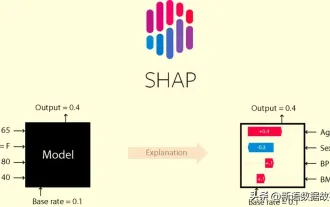 This article will take you to understand SHAP: model explanation for machine learning
Jun 01, 2024 am 10:58 AM
This article will take you to understand SHAP: model explanation for machine learning
Jun 01, 2024 am 10:58 AM
In the fields of machine learning and data science, model interpretability has always been a focus of researchers and practitioners. With the widespread application of complex models such as deep learning and ensemble methods, understanding the model's decision-making process has become particularly important. Explainable AI|XAI helps build trust and confidence in machine learning models by increasing the transparency of the model. Improving model transparency can be achieved through methods such as the widespread use of multiple complex models, as well as the decision-making processes used to explain the models. These methods include feature importance analysis, model prediction interval estimation, local interpretability algorithms, etc. Feature importance analysis can explain the decision-making process of a model by evaluating the degree of influence of the model on the input features. Model prediction interval estimate
 Transparent! An in-depth analysis of the principles of major machine learning models!
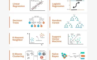
Apr 12, 2024 pm 05:55 PM
Transparent! An in-depth analysis of the principles of major machine learning models!
Apr 12, 2024 pm 05:55 PM
In layman’s terms, a machine learning model is a mathematical function that maps input data to a predicted output. More specifically, a machine learning model is a mathematical function that adjusts model parameters by learning from training data to minimize the error between the predicted output and the true label. There are many models in machine learning, such as logistic regression models, decision tree models, support vector machine models, etc. Each model has its applicable data types and problem types. At the same time, there are many commonalities between different models, or there is a hidden path for model evolution. Taking the connectionist perceptron as an example, by increasing the number of hidden layers of the perceptron, we can transform it into a deep neural network. If a kernel function is added to the perceptron, it can be converted into an SVM. this one
 Identify overfitting and underfitting through learning curves
Apr 29, 2024 pm 06:50 PM
Identify overfitting and underfitting through learning curves
Apr 29, 2024 pm 06:50 PM
This article will introduce how to effectively identify overfitting and underfitting in machine learning models through learning curves. Underfitting and overfitting 1. Overfitting If a model is overtrained on the data so that it learns noise from it, then the model is said to be overfitting. An overfitted model learns every example so perfectly that it will misclassify an unseen/new example. For an overfitted model, we will get a perfect/near-perfect training set score and a terrible validation set/test score. Slightly modified: "Cause of overfitting: Use a complex model to solve a simple problem and extract noise from the data. Because a small data set as a training set may not represent the correct representation of all data." 2. Underfitting Heru
 The evolution of artificial intelligence in space exploration and human settlement engineering
Apr 29, 2024 pm 03:25 PM
The evolution of artificial intelligence in space exploration and human settlement engineering
Apr 29, 2024 pm 03:25 PM
In the 1950s, artificial intelligence (AI) was born. That's when researchers discovered that machines could perform human-like tasks, such as thinking. Later, in the 1960s, the U.S. Department of Defense funded artificial intelligence and established laboratories for further development. Researchers are finding applications for artificial intelligence in many areas, such as space exploration and survival in extreme environments. Space exploration is the study of the universe, which covers the entire universe beyond the earth. Space is classified as an extreme environment because its conditions are different from those on Earth. To survive in space, many factors must be considered and precautions must be taken. Scientists and researchers believe that exploring space and understanding the current state of everything can help understand how the universe works and prepare for potential environmental crises
 Implementing Machine Learning Algorithms in C++: Common Challenges and Solutions
Jun 03, 2024 pm 01:25 PM
Implementing Machine Learning Algorithms in C++: Common Challenges and Solutions
Jun 03, 2024 pm 01:25 PM
Common challenges faced by machine learning algorithms in C++ include memory management, multi-threading, performance optimization, and maintainability. Solutions include using smart pointers, modern threading libraries, SIMD instructions and third-party libraries, as well as following coding style guidelines and using automation tools. Practical cases show how to use the Eigen library to implement linear regression algorithms, effectively manage memory and use high-performance matrix operations.
 Explainable AI: Explaining complex AI/ML models
Jun 03, 2024 pm 10:08 PM
Explainable AI: Explaining complex AI/ML models
Jun 03, 2024 pm 10:08 PM
Translator | Reviewed by Li Rui | Chonglou Artificial intelligence (AI) and machine learning (ML) models are becoming increasingly complex today, and the output produced by these models is a black box – unable to be explained to stakeholders. Explainable AI (XAI) aims to solve this problem by enabling stakeholders to understand how these models work, ensuring they understand how these models actually make decisions, and ensuring transparency in AI systems, Trust and accountability to address this issue. This article explores various explainable artificial intelligence (XAI) techniques to illustrate their underlying principles. Several reasons why explainable AI is crucial Trust and transparency: For AI systems to be widely accepted and trusted, users need to understand how decisions are made
 Is Flash Attention stable? Meta and Harvard found that their model weight deviations fluctuated by orders of magnitude
May 30, 2024 pm 01:24 PM
Is Flash Attention stable? Meta and Harvard found that their model weight deviations fluctuated by orders of magnitude
May 30, 2024 pm 01:24 PM
MetaFAIR teamed up with Harvard to provide a new research framework for optimizing the data bias generated when large-scale machine learning is performed. It is known that the training of large language models often takes months and uses hundreds or even thousands of GPUs. Taking the LLaMA270B model as an example, its training requires a total of 1,720,320 GPU hours. Training large models presents unique systemic challenges due to the scale and complexity of these workloads. Recently, many institutions have reported instability in the training process when training SOTA generative AI models. They usually appear in the form of loss spikes. For example, Google's PaLM model experienced up to 20 loss spikes during the training process. Numerical bias is the root cause of this training inaccuracy,
