 Technology peripherals
 AI
AI
 Abandon the encoder-decoder architecture and use the diffusion model for edge detection, which is more effective. The National University of Defense Technology proposed DiffusionEdge
Abandon the encoder-decoder architecture and use the diffusion model for edge detection, which is more effective. The National University of Defense Technology proposed DiffusionEdge
Current deep edge detection networks usually adopt an encoder-decoder architecture, which contains up and down sampling modules to better extract multi-level features. However, this structure limits the network to output accurate and detailed edge detection results.
In response to this problem, a paper at AAAI 2024 provides a new solution.

- ##Thesis title: DiffusionEdge: Diffusion Probabilistic Model for Crisp Edge Detection
- Authors: Ye Yunfan (National University of Defense Technology), Xu Kai (National University of Defense Technology), Huang Yuxing (National University of Defense Technology), Yi Renjiao (National University of Defense Technology), Cai Zhiping (National University of Defense Technology)
- Paper link: https://arxiv.org/abs/2401.02032
- Open source code: https://github.com/GuHuangAI/DiffusionEdge
iGRAPE Lab of the National University of Defense Technology proposed a new method for the two-dimensional edge detection task. This method utilizes a diffusion probability model to generate edge result maps during a learning iterative denoising process. In order to reduce the consumption of computing resources, this method uses latent space to train the network and introduces an uncertainty distillation module to optimize performance. At the same time, this method also adopts a decoupled architecture to accelerate the denoising process and introduces an adaptive Fourier filter to adjust the features. With these designs, the method is able to train stably with limited resources and predict clear and accurate edge maps with fewer augmentation strategies. Experimental results show that this method significantly outperforms other methods in terms of accuracy and precision on four public benchmark datasets.
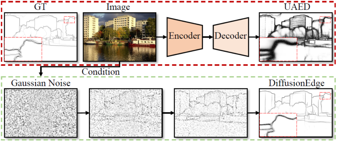
Figure 1 Example of edge detection process and advantages based on diffusion probability model
The innovation of this article Including:
Proposed a diffusion model DiffusionEdge for edge detection tasks, which can predict finer and more accurate edge maps without post-processing.
In order to solve the difficulties in applying the diffusion model, we have designed a variety of techniques to ensure that the method learns stably in the latent space. At the same time, we also retain pixel-level uncertainty prior knowledge and adaptively filter latent features in Fourier space.
3. Extensive comparative experiments conducted on four edge detection public benchmark data sets demonstrate that DiffusionEdge has excellent performance advantages in terms of accuracy and fineness.
Related work
Methods based on deep learning usually adopt a codec structure containing up and down sampling to integrate multi-layer features [1-2], Or integrate the uncertainty information of multiple annotations to improve the accuracy of edge detection [3]. However, naturally limited by such a structure, the edge result map generated is too thick for downstream tasks and relies heavily on post-processing. The problem still needs to be solved. Although many works have been explored in loss functions [4-5] and label correction strategies [6] to enable the network to output finer edges, this paper believes that this field still needs a method that can be used without any additional modules. Edge detectors that directly meet accuracy and fineness without any post-processing steps.
The diffusion model is a type of generative model based on Markov chain, which gradually restores the target data sample through the learning denoising process. Diffusion models have shown excellent performance in areas such as computer vision, natural language processing, and audio generation. Not only that, by using images or other modal inputs as additional conditions, it also shows great potential in perception tasks, such as image segmentation [7], target detection [8] and attitude estimation [9], etc. .
Method Description
The overall framework of the DiffusionEdge method proposed in this article is shown in Figure 2. Inspired by previous work, this method trains a diffusion model with decoupled structure in latent space and inputs images as additional conditional cues. This method introduces an adaptive Fourier filter for frequency analysis, and in order to retain pixel-level uncertainty information from multiple annotators and reduce requirements on computing resources, it also directly uses cross-entropy loss optimization in a distilled manner. Hidden space.
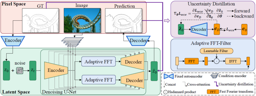
Figure 2 The overall structure of DiffusionEdge
As the current diffusion model is plagued by problems such as too many sampling steps and too long inference time, this method is influenced by DDM Inspired by [10], the decoupled diffusion model architecture is also used to accelerate the sampling inference process. Among them, the decoupled forward diffusion process is controlled by a combination of explicit transition probability and standard Wiener process:

where  and
and  represents the initial edge and noise edge respectively,
  refers to the explicit conversion function of the reverse edge gradient. Similar to DDM, this method uses the constant function
  by default, and its corresponding inverse process can be expressed as:

where . In order to train the decoupled diffusion model, the method requires simultaneous supervision of the data and noise components, therefore, the training objective can be parameterized as:

##where is the parameter in the denoising network. Since the diffusion model will take up too much computational cost if it is trained in the original image space, referring to the idea of [11], the method proposed in this paper transfers the training process to a latent space with 4 times the size of the downsampling space. 
As shown in Figure 2, this method first trains a pair of autoencoder and decoder networks. The encoder compresses the edge annotation into a latent variable, while the decoder Used to recover the original edge label from this latent variable. In this way, during the training stage of the denoising network based on the U-Net structure, this method fixes the weight of the pair of autoencoder and decoder networks, and trains the denoising process in the latent space, which can greatly reduce the computational cost of the network. consumption of resources while maintaining good performance.
In order to improve the final performance of the network, the method proposed in this article introduces a module that can adaptively filter out different frequency features in the decoupling operation. As shown in the lower left corner of Figure 2, this method integrates the adaptive fast Fourier transform filter (Adaptive FFT-filter) into the denoising Unet network before the decoupling operation to adaptively filter and separate in the frequency domain. Out edge map and noise components. Specifically, given the encoder feature  , the method first performs a two-dimensional Fourier transform (FFT) along the spatial dimension and represents the transformed feature as
  . Next, in order to train this adaptive spectrum filtering module, a learnable weight map
  is constructed and its W is multiplied by Fc. Spectral filters can globally adjust specific frequencies, and the learned weights can be adapted to different frequency cases of target distributions in different datasets. By adaptively filtering out unwanted components, this method maps features from the frequency domain back to the spatial domain through an inverse fast Fourier transform (IFFT) operation. Finally, by additionally introducing the residual connection from , we avoid completely filtering out all useful information. The above process can be described by the following formula:

where  is the output feature and o represents the Hadamard Product.
Since the number of edge and non-edge pixels is highly unbalanced (most pixels are non-edge background), referring to previous work, we also introduce an uncertainty-aware loss function. train. Specifically, as the true value edge probability of the i-th pixel, for the i-th pixel in the j-th edge map, its value is 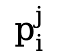 , then the uncertainty-aware WCE loss is calculated as follows:

where , where
  is the threshold that determines the uncertain edge pixels in the true value annotation. If the pixel value is greater than 0 and less than this threshold, then this type of blur is not confident enough. Pixel samples will be ignored in subsequent optimization processes (loss function is 0).
  and
and  respectively represent the number of edge and non-edge pixels in the ground truth annotated edge map. is used to balance the weight of
  and
and  (set to 1.1). Therefore, the final loss function for each edge map is calculated as
 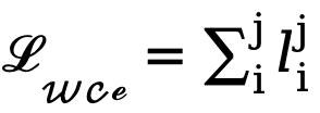 .
.
Ignoring blurry low-confidence pixels during the optimization process can avoid network confusion, make the training process converge more stably, and improve the performance of the model. However, it is almost impossible to directly apply the binary cross-entropy loss in a latent space that is both numerically and spatially misaligned. In particular, the uncertainty-aware cross-entropy loss uses a threshold (generally from 0 to 1) to determine whether a pixel is an edge, which is defined from the image space, while the latent variable follows a normal distribution and has complete Different scope and practical significance. Furthermore, pixel-level uncertainty is difficult to reconcile with different sizes of encoded and downsampled latent features, and the two are not directly compatible. Therefore, directly applying cross-entropy loss to optimize latent variables inevitably leads to incorrect uncertainty perception. 
On the other hand, one can choose to decode the latent variables back to the image level, thus directly supervising the predicted edge result map using an uncertainty-aware cross-entropy loss. Unfortunately, this implementation allows the backpropagated parameter gradients to pass through the redundant autoencoder network, making it difficult to effectively transfer the gradients. In addition, additional gradient calculations in the autoencoder network will bring huge GPU memory consumption costs, which violates the original intention of this method to design a practical edge detector and is difficult to generalize to practical applications. Therefore, this method proposes uncertainty distillation loss, which can directly optimize the gradient on the latent space. Specifically, assuming that the reconstructed latent variable is , the decoder of the autoencoder network is D, and the decoded The edge result is eD. This method considers directly calculating the gradient of the uncertainty-aware binary cross-entropy loss  based on the chain rule. The specific calculation method is:

In order to eliminate the negative impact of the autoencoder network, this method directly skips the autoencoder to pass the gradient and adjusts the calculation method of the gradient  to:
to: 

# Such an implementation greatly reduces the computational cost and allows direct optimization on latent variables using uncertainty-aware loss functions. In this way, combined with a time-varying loss weight that changes adaptively with the number of steps t, the final training optimization goal of this method can be expressed as:

Experimental results
This method was tested on public standard data sets for edge detection that are widely used in four fields: BSDS, NYUDv2, Multicue and BIPED. Since it is difficult to label edge detection data and the amount of labeled data is relatively small, previous methods usually use various strategies to enhance the data set. For example, images in BSDS are enhanced by horizontal flipping (2×), scaling (3×), and rotation (16×), resulting in a training set that is 96 times larger than the original version. Common enhancement strategies used by previous methods on other datasets are summarized in Table 1, where F stands for horizontal flip, S stands for scaling, R stands for rotation, C stands for cropping, and G stands for gamma correction. The difference is that this method only needs to use randomly cropped image patches of 320320 to train all data. In the BSDS data set, this method only uses random flipping and scaling, and its quantitative comparison results are shown in Table 2. In the NYUDv2, Multicue and BIPED datasets, the method only needs to be trained with random flips. With fewer enhancement strategies, this method performs better than previous methods on various data sets and various indicators. By observing the prediction results in Figure 3-5, we can see that DiffusionEdge can learn and predict edge detection results that are almost the same as the gt distribution. The advantage of accurate and clear prediction results is very important for downstream tasks that require refinement. , and also demonstrated its great potential to be directly applied to subsequent tasks.
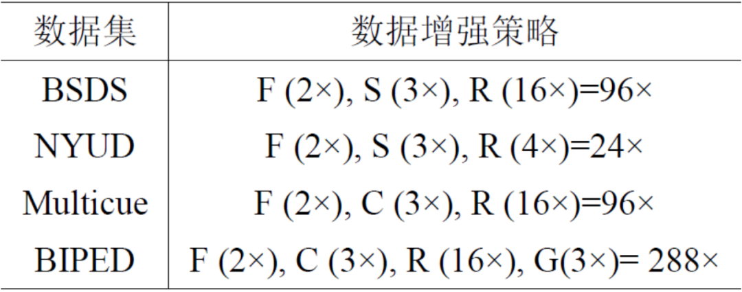
Table 1 Enhancement strategies used by previous methods on four edge detection data sets
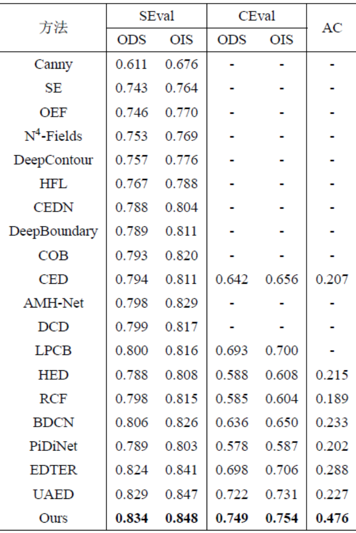
Table 2 Quantitative comparison of different methods on the BSDS data set
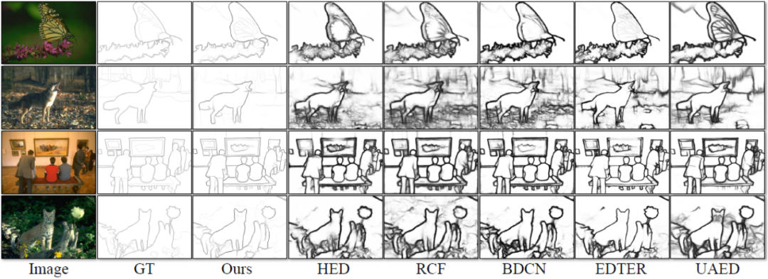
Figure 3 Different methods on the BSDS data set Qualitative comparison
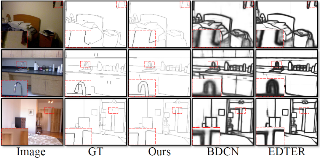
Figure 4 Qualitative comparison of different methods on the NYUDv2 data set
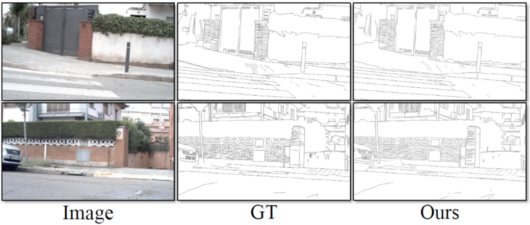
Figure 5 Qualitative comparison of different methods on the BIPED data set
The above is the detailed content of Abandon the encoder-decoder architecture and use the diffusion model for edge detection, which is more effective. The National University of Defense Technology proposed DiffusionEdge. For more information, please follow other related articles on the PHP Chinese website!

Hot AI Tools

Undresser.AI Undress
AI-powered app for creating realistic nude photos

AI Clothes Remover
Online AI tool for removing clothes from photos.

Undress AI Tool
Undress images for free

Clothoff.io
AI clothes remover

AI Hentai Generator
Generate AI Hentai for free.

Hot Article

Hot Tools

Notepad++7.3.1
Easy-to-use and free code editor

SublimeText3 Chinese version
Chinese version, very easy to use

Zend Studio 13.0.1
Powerful PHP integrated development environment

Dreamweaver CS6
Visual web development tools

SublimeText3 Mac version
God-level code editing software (SublimeText3)

Hot Topics
 1378
1378
 52
52
 How to implement file sorting by debian readdir
Apr 13, 2025 am 09:06 AM
In Debian systems, the readdir function is used to read directory contents, but the order in which it returns is not predefined. To sort files in a directory, you need to read all files first, and then sort them using the qsort function. The following code demonstrates how to sort directory files using readdir and qsort in Debian system: #include#include#include#include#include//Custom comparison function, used for qsortintcompare(constvoid*a,constvoid*b){returnstrcmp(*(
 How to optimize the performance of debian readdir
Apr 13, 2025 am 08:48 AM
In Debian systems, readdir system calls are used to read directory contents. If its performance is not good, try the following optimization strategy: Simplify the number of directory files: Split large directories into multiple small directories as much as possible, reducing the number of items processed per readdir call. Enable directory content caching: build a cache mechanism, update the cache regularly or when directory content changes, and reduce frequent calls to readdir. Memory caches (such as Memcached or Redis) or local caches (such as files or databases) can be considered. Adopt efficient data structure: If you implement directory traversal by yourself, select more efficient data structures (such as hash tables instead of linear search) to store and access directory information
 How debian readdir integrates with other tools
Apr 13, 2025 am 09:42 AM
The readdir function in the Debian system is a system call used to read directory contents and is often used in C programming. This article will explain how to integrate readdir with other tools to enhance its functionality. Method 1: Combining C language program and pipeline First, write a C program to call the readdir function and output the result: #include#include#include#includeintmain(intargc,char*argv[]){DIR*dir;structdirent*entry;if(argc!=2){
 Debian mail server firewall configuration tips
Apr 13, 2025 am 11:42 AM
Configuring a Debian mail server's firewall is an important step in ensuring server security. The following are several commonly used firewall configuration methods, including the use of iptables and firewalld. Use iptables to configure firewall to install iptables (if not already installed): sudoapt-getupdatesudoapt-getinstalliptablesView current iptables rules: sudoiptables-L configuration
 How to configure firewall rules for Debian syslog
Apr 13, 2025 am 06:51 AM
This article describes how to configure firewall rules using iptables or ufw in Debian systems and use Syslog to record firewall activities. Method 1: Use iptablesiptables is a powerful command line firewall tool in Debian system. View existing rules: Use the following command to view the current iptables rules: sudoiptables-L-n-v allows specific IP access: For example, allow IP address 192.168.1.100 to access port 80: sudoiptables-AINPUT-ptcp--dport80-s192.16
 How to set the Debian Apache log level
Apr 13, 2025 am 08:33 AM
This article describes how to adjust the logging level of the ApacheWeb server in the Debian system. By modifying the configuration file, you can control the verbose level of log information recorded by Apache. Method 1: Modify the main configuration file to locate the configuration file: The configuration file of Apache2.x is usually located in the /etc/apache2/ directory. The file name may be apache2.conf or httpd.conf, depending on your installation method. Edit configuration file: Open configuration file with root permissions using a text editor (such as nano): sudonano/etc/apache2/apache2.conf
 How to learn Debian syslog
Apr 13, 2025 am 11:51 AM
This guide will guide you to learn how to use Syslog in Debian systems. Syslog is a key service in Linux systems for logging system and application log messages. It helps administrators monitor and analyze system activity to quickly identify and resolve problems. 1. Basic knowledge of Syslog The core functions of Syslog include: centrally collecting and managing log messages; supporting multiple log output formats and target locations (such as files or networks); providing real-time log viewing and filtering functions. 2. Install and configure Syslog (using Rsyslog) The Debian system uses Rsyslog by default. You can install it with the following command: sudoaptupdatesud
 How Debian OpenSSL prevents man-in-the-middle attacks
Apr 13, 2025 am 10:30 AM
In Debian systems, OpenSSL is an important library for encryption, decryption and certificate management. To prevent a man-in-the-middle attack (MITM), the following measures can be taken: Use HTTPS: Ensure that all network requests use the HTTPS protocol instead of HTTP. HTTPS uses TLS (Transport Layer Security Protocol) to encrypt communication data to ensure that the data is not stolen or tampered during transmission. Verify server certificate: Manually verify the server certificate on the client to ensure it is trustworthy. The server can be manually verified through the delegate method of URLSession


