

How to sum cells in multiple worksheets in Excel

This article will demonstrate how to sum cells in multiple worksheets in Excel. Microsoft Excel is a powerful spreadsheet program used for data management. When working with data, you may need to sum across multiple cells. This guide will show you how to achieve this easily.
How to sum cells in multiple worksheets in Excel
When summing cells in multiple worksheets in Excel, you may encounter the following two situations:
- Add a single cell value
- Add values in cell range
We will introduce both methods here.
Add a single cell value across multiple worksheets in Excel
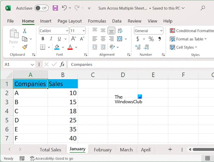
We collected sample data containing the sales of 6 different companies in four consecutive months (from January to April). The total sales table includes each company's total sales during the four-month period.
To sum the data in all worksheets, use the following formula:
=SUM(第一张图纸名称:最后一张图纸名称!单元格地址)
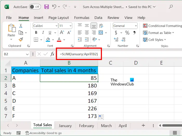
In this formula, the colon indicates the range of the plate. In our example, we will sum the values from all tables for different companies. Therefore, the formula will be:
=SUM(1月:4月B2)
If the drawing name contains spaces, such as Drawing 1, the drawing name must be typed under single quotes. For example:
=SUM(‘Sheet 1:Sheet 4’!B2)
In the above formula, cell B2 represents the sales volume of company A. Please enter the correct cell address or you will receive an error message.
Alternatively, you can try this.
When finished, use the fill handles to fill the formula in all cells.
Add single cell value in selected worksheet in Excel
If you want to add the values in some selected worksheets in Excel, you cannot use the above formula because it contains colons. In this case, you must use commas to separate the different worksheets you want to add.
In this case you can use the following formula:
=SUM(表%1!单元格地址,表%2!单元格地址,表%3!单元格地址,...)
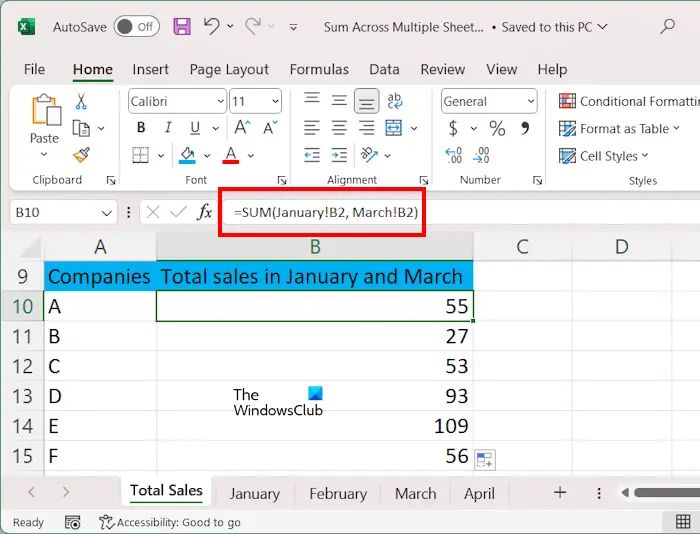
For example, in our example, we want to display the total sales of different companies in January and March, the formula is:
=SUM(1月B2,3月B2)
In the above formula, B2 represents the cell address. If there are spaces in the drawing name, type its name within single quotes, for example:
=SUM(‘Sheet 1’!B2,‘Sheet 3’!B2)
Alternatively, you can follow these steps:
When finished, use the fill handles to copy the formula to all cells.
Add values in a cell range in multiple worksheets in Excel
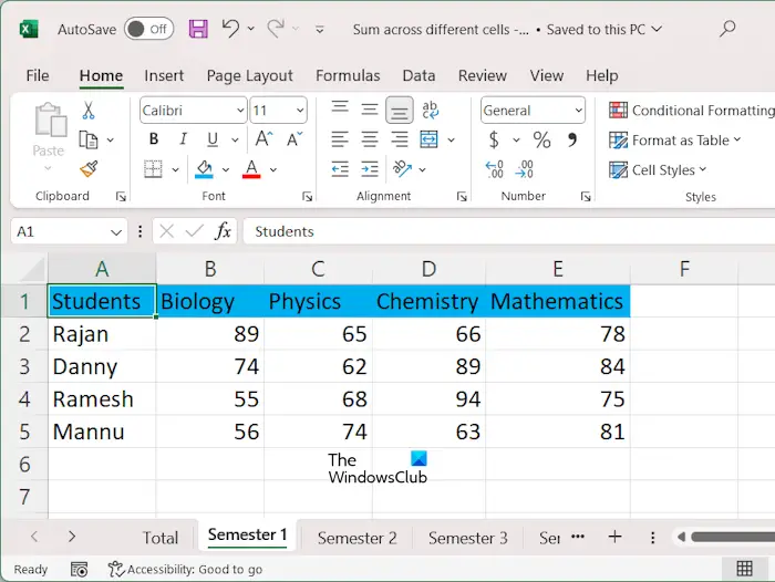
If your data contains multiple values in different cells in different worksheets, you can also add these values by selecting a range of cells. To explain this, we created another sample data containing the grades of students in different subjects in different semesters.
To sum data in a range of cells on different worksheets, use the following formula:
=SUM(第一个工作表名称:最后一个工作表名称!单元格区域)
In our example, if we want to add points in all subjects in all semesters, the formula will be:
=sum(‘第一学期:第四学期’!B2:E2)
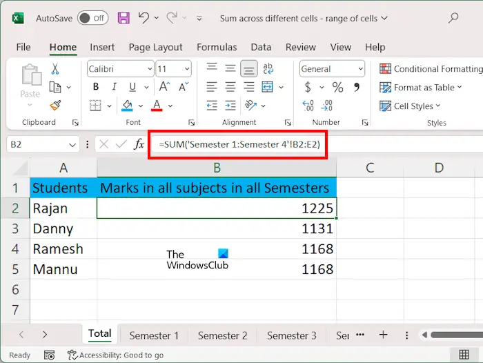
在上式中,学期1:学期4表示片材的范围,B2:E2表示单元格的范围。我们在公式中使用了单引号,因为我们的工作表名称包含空格。
在Excel中的选定工作表的单元格区域中添加值
要在Excel中对选定工作表的单元格范围内的值求和,请使用以下公式:
=SUM(表1!单元格范围,第二页!单元格范围第三页!单元格范围,.)
假设我们要显示第二学期和第四学期不同科目学生的总分,公式为:
=sum(‘学期2’!B2:E2,‘学期4’!B2:E2)
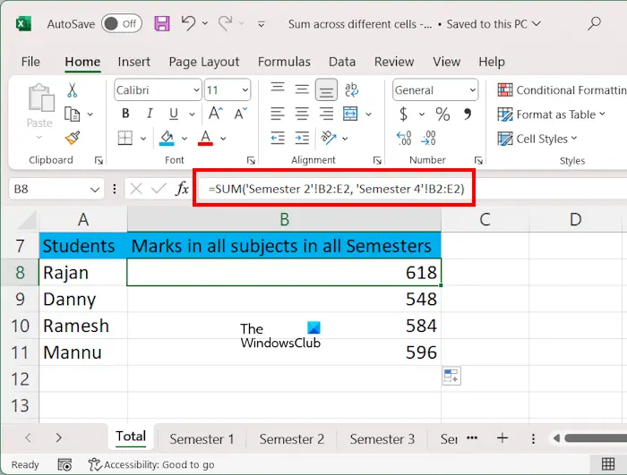
最简单的方法是分别选择每个工作表中的单元格范围。如果在所有工作表中添加单元格区域,则可以使用Shift键。我们已经在本文前面解释了执行此操作的步骤。完成后,使用填充手柄将公式复制到剩余的单元格。
如何在求和中添加多行?
您可以使用求和公式在Excel中添加多行。公式结构为=SUM(第一行单元格区域,第二行单元格区域,第三行单元格区域,…)。或者,您可以用鼠标选择不同行中的单元格范围,并用逗号分隔它们。
如何在Google Sheets中添加多行的总和?
在Google Sheets中添加多行的公式与在Excel中使用的公式相同。类型=SUM(第一行单元格范围,第二行单元格范围,第三行单元格范围,…)然后按Enter键。Google Sheets将显示总和。
Read next: How to remove Formula in Excel and keep Text.
The above is the detailed content of How to sum cells in multiple worksheets in Excel. For more information, please follow other related articles on the PHP Chinese website!

Hot AI Tools

Undresser.AI Undress
AI-powered app for creating realistic nude photos

AI Clothes Remover
Online AI tool for removing clothes from photos.

Undress AI Tool
Undress images for free

Clothoff.io
AI clothes remover

AI Hentai Generator
Generate AI Hentai for free.

Hot Article
Hot Tools

Notepad++7.3.1
Easy-to-use and free code editor

SublimeText3 Chinese version
Chinese version, very easy to use

Zend Studio 13.0.1
Powerful PHP integrated development environment

Dreamweaver CS6
Visual web development tools

SublimeText3 Mac version
God-level code editing software (SublimeText3)
Hot Topics


 What should I do if the frame line disappears when printing in Excel?
Mar 21, 2024 am 09:50 AM
What should I do if the frame line disappears when printing in Excel?
Mar 21, 2024 am 09:50 AM
If when opening a file that needs to be printed, we will find that the table frame line has disappeared for some reason in the print preview. When encountering such a situation, we must deal with it in time. If this also appears in your print file If you have questions like this, then join the editor to learn the following course: What should I do if the frame line disappears when printing a table in Excel? 1. Open a file that needs to be printed, as shown in the figure below. 2. Select all required content areas, as shown in the figure below. 3. Right-click the mouse and select the "Format Cells" option, as shown in the figure below. 4. Click the “Border” option at the top of the window, as shown in the figure below. 5. Select the thin solid line pattern in the line style on the left, as shown in the figure below. 6. Select "Outer Border"
 How to filter more than 3 keywords at the same time in excel
Mar 21, 2024 pm 03:16 PM
How to filter more than 3 keywords at the same time in excel
Mar 21, 2024 pm 03:16 PM
Excel is often used to process data in daily office work, and it is often necessary to use the "filter" function. When we choose to perform "filtering" in Excel, we can only filter up to two conditions for the same column. So, do you know how to filter more than 3 keywords at the same time in Excel? Next, let me demonstrate it to you. The first method is to gradually add the conditions to the filter. If you want to filter out three qualifying details at the same time, you first need to filter out one of them step by step. At the beginning, you can first filter out employees with the surname "Wang" based on the conditions. Then click [OK], and then check [Add current selection to filter] in the filter results. The steps are as follows. Similarly, perform filtering separately again
 How to change excel table compatibility mode to normal mode
Mar 20, 2024 pm 08:01 PM
How to change excel table compatibility mode to normal mode
Mar 20, 2024 pm 08:01 PM
In our daily work and study, we copy Excel files from others, open them to add content or re-edit them, and then save them. Sometimes a compatibility check dialog box will appear, which is very troublesome. I don’t know Excel software. , can it be changed to normal mode? So below, the editor will bring you detailed steps to solve this problem, let us learn together. Finally, be sure to remember to save it. 1. Open a worksheet and display an additional compatibility mode in the name of the worksheet, as shown in the figure. 2. In this worksheet, after modifying the content and saving it, the dialog box of the compatibility checker always pops up. It is very troublesome to see this page, as shown in the figure. 3. Click the Office button, click Save As, and then
 How to type subscript in excel
Mar 20, 2024 am 11:31 AM
How to type subscript in excel
Mar 20, 2024 am 11:31 AM
eWe often use Excel to make some data tables and the like. Sometimes when entering parameter values, we need to superscript or subscript a certain number. For example, mathematical formulas are often used. So how do you type the subscript in Excel? ?Let’s take a look at the detailed steps: 1. Superscript method: 1. First, enter a3 (3 is superscript) in Excel. 2. Select the number "3", right-click and select "Format Cells". 3. Click "Superscript" and then "OK". 4. Look, the effect is like this. 2. Subscript method: 1. Similar to the superscript setting method, enter "ln310" (3 is the subscript) in the cell, select the number "3", right-click and select "Format Cells". 2. Check "Subscript" and click "OK"
 How to set superscript in excel
Mar 20, 2024 pm 04:30 PM
How to set superscript in excel
Mar 20, 2024 pm 04:30 PM
When processing data, sometimes we encounter data that contains various symbols such as multiples, temperatures, etc. Do you know how to set superscripts in Excel? When we use Excel to process data, if we do not set superscripts, it will make it more troublesome to enter a lot of our data. Today, the editor will bring you the specific setting method of excel superscript. 1. First, let us open the Microsoft Office Excel document on the desktop and select the text that needs to be modified into superscript, as shown in the figure. 2. Then, right-click and select the "Format Cells" option in the menu that appears after clicking, as shown in the figure. 3. Next, in the “Format Cells” dialog box that pops up automatically
 How to use the iif function in excel
Mar 20, 2024 pm 06:10 PM
How to use the iif function in excel
Mar 20, 2024 pm 06:10 PM
Most users use Excel to process table data. In fact, Excel also has a VBA program. Apart from experts, not many users have used this function. The iif function is often used when writing in VBA. It is actually the same as if The functions of the functions are similar. Let me introduce to you the usage of the iif function. There are iif functions in SQL statements and VBA code in Excel. The iif function is similar to the IF function in the excel worksheet. It performs true and false value judgment and returns different results based on the logically calculated true and false values. IF function usage is (condition, yes, no). IF statement and IIF function in VBA. The former IF statement is a control statement that can execute different statements according to conditions. The latter
 Where to set excel reading mode
Mar 21, 2024 am 08:40 AM
Where to set excel reading mode
Mar 21, 2024 am 08:40 AM
In the study of software, we are accustomed to using excel, not only because it is convenient, but also because it can meet a variety of formats needed in actual work, and excel is very flexible to use, and there is a mode that is convenient for reading. Today I brought For everyone: where to set the excel reading mode. 1. Turn on the computer, then open the Excel application and find the target data. 2. There are two ways to set the reading mode in Excel. The first one: In Excel, there are a large number of convenient processing methods distributed in the Excel layout. In the lower right corner of Excel, there is a shortcut to set the reading mode. Find the pattern of the cross mark and click it to enter the reading mode. There is a small three-dimensional mark on the right side of the cross mark.
 How to insert excel icons into PPT slides
Mar 26, 2024 pm 05:40 PM
How to insert excel icons into PPT slides
Mar 26, 2024 pm 05:40 PM
1. Open the PPT and turn the page to the page where you need to insert the excel icon. Click the Insert tab. 2. Click [Object]. 3. The following dialog box will pop up. 4. Click [Create from file] and click [Browse]. 5. Select the excel table to be inserted. 6. Click OK and the following page will pop up. 7. Check [Show as icon]. 8. Click OK.
