

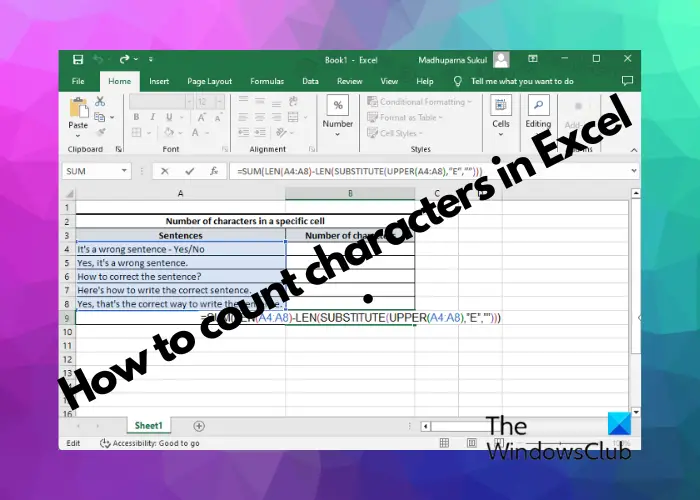
How to count characters in Microsoft Excel

Although Excel is primarily used for working with numeric data, you can also include text in cells. So, if you need to transfer data in Excel and limit the number of characters in a cell, you may need to know how to calculate the number of characters.
With these factors in mind, we wrote this article to share some practical tips to help you count characters in Microsoft Excel as easily as you count words.
How to count characters in Microsoft Excel
Although you may need to count characters in a single cell, in real life you may also need to perform the same operation on multiple cells or ranges of cells. We provide detailed guides to help you handle character calculations and operations in Microsoft Excel.
1]Use the LEN formula to calculate the number of characters
For a single cell
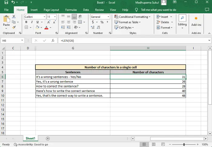
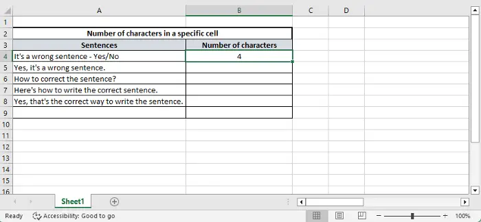
In Excel, to count the number of characters in a single cell, you can use the text function LEN. Although the syntax is LEN(cell), the exact formula is used to count the number of characters.
=LEN(单元格)
Replace (Cell) with the cell reference whose characters you want to count. So, for example, if you want to count the number of characters in cell G6 (as shown in the image above), the formula would be:
=LEN(G6)
Please note that in Microsoft Excel, all punctuation marks, spaces, and even punctuation marks after a string are counted as characters in the sentence.
Also, to calculate the number of bytes in a cell, you can use the LENB function, such as =LENB(A2).
For multiple communities
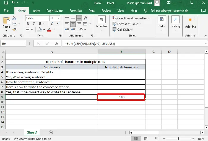
However, if you want to count the total number of characters in multiple cells, you can use the following formula to get the result:
=SUM(LEN(cell1),LEN(cell2),LEN(cell3))
So, in this example, you need to use the LEN function for all the cells whose characters you want to count, and add the SUM function to them.
For example, if you want to count the total number of characters in cells A4, A6, and A8, the formula would look like this:
=SUM(LEN(A4)、LEN(A6)、LEN(A8))
Read: How to convert numbers stored as text to numbers in Excel
2] Count characters within a single/multiple cell range
Single cell range formula
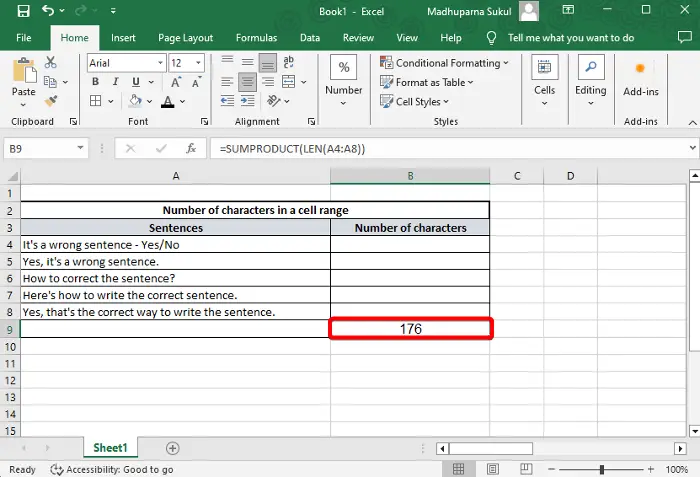
However, if you want to count characters in adjacent (adjacent) cell ranges, there are two methods. While the above formula can also help you easily count the number of characters in a range of cells, using the formula below can also help you quickly achieve the same calculation. So, for example, to count the total number of characters in cells A4 through A8, the formula would look like this:
=SUM(镜头(A4:A8))
Alternatively, you can use the following formula to achieve the same results:
=SUMPRODUCT(LEN(A4:A8))
Multiple cell range formulas
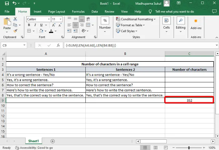
However, if you want to know the total number of characters in multiple cell ranges (for example, from A4 to A8 and from B4 to B8), you can use the following formula:
=SUM(镜头(A4:A8),镜头(B4:B8))

或

=SUMPRODUCT(LEN(A4:A8),LEN(B4:B8))
Read: How to circle numbers in Excel
3] Count specific characters in Excel
For specific characters in Excel
Sometimes, after adding text to a cell in Excel, you may need to count the total number of specific characters in that specific cell. In this case you can use LEN with the replacement function. So, for example, if you want to count the number of E's in cell A4, the formula would look like this:
=LEN(A4)-LEN(SUBSTITUTE(A4,“e”,"”))
Here, replacement is case-sensitive. So if you enter letters in lower case it will return results accordingly and vice versa.
However, you can also choose to ignore letter case, you can use the following formula in the above format:
=LEN(A4)-LEN(替换(UPER(A4),“E”,“”))
For specific characters in a range of cells,
Now, to count the total number of characters in a range of cells, you need to use all three functions: LEN, SUM, and SUB. So, for example, if you want to count the number of a specific character, such as E, in the cell range A4 to A8, the formula would look like this:
=sum(LEN(A4:A8)-LEN(替换(UPPER(A4:A8),“E”,“”))
Read: How to spell check a specific range, part, cell or column in Excel
How to count the number of texts in Excel?
To count the number of cells containing text in Excel, you can use the formula =COUNTIF(Range, "*"). You can then replace that range with the range of cells you want to calculate. This formula counts all cells within the specified range that contain text. It ensures accurate data management and analysis.
What is the formula to calculate LEN in Excel?
The formula for LEN in Excel is =LEN(text), where text illustrates the cell reference or string you want to measure. This formula generates the total count of characters present, which includes spaces and punctuation marks, in the specified cell's content. For instance, =LEN(A1) counts the character count in cell A1.
The above is the detailed content of How to count characters in Microsoft Excel. For more information, please follow other related articles on the PHP Chinese website!

Hot AI Tools

Undresser.AI Undress
AI-powered app for creating realistic nude photos

AI Clothes Remover
Online AI tool for removing clothes from photos.

Undress AI Tool
Undress images for free

Clothoff.io
AI clothes remover

AI Hentai Generator
Generate AI Hentai for free.

Hot Article
Hot Tools

Notepad++7.3.1
Easy-to-use and free code editor

SublimeText3 Chinese version
Chinese version, very easy to use

Zend Studio 13.0.1
Powerful PHP integrated development environment

Dreamweaver CS6
Visual web development tools

SublimeText3 Mac version
God-level code editing software (SublimeText3)
Hot Topics
 1382
1382
 52
52

 What should I do if the frame line disappears when printing in Excel?
Mar 21, 2024 am 09:50 AM
What should I do if the frame line disappears when printing in Excel?
Mar 21, 2024 am 09:50 AM
If when opening a file that needs to be printed, we will find that the table frame line has disappeared for some reason in the print preview. When encountering such a situation, we must deal with it in time. If this also appears in your print file If you have questions like this, then join the editor to learn the following course: What should I do if the frame line disappears when printing a table in Excel? 1. Open a file that needs to be printed, as shown in the figure below. 2. Select all required content areas, as shown in the figure below. 3. Right-click the mouse and select the "Format Cells" option, as shown in the figure below. 4. Click the “Border” option at the top of the window, as shown in the figure below. 5. Select the thin solid line pattern in the line style on the left, as shown in the figure below. 6. Select "Outer Border"
 How to filter more than 3 keywords at the same time in excel
Mar 21, 2024 pm 03:16 PM
How to filter more than 3 keywords at the same time in excel
Mar 21, 2024 pm 03:16 PM
Excel is often used to process data in daily office work, and it is often necessary to use the "filter" function. When we choose to perform "filtering" in Excel, we can only filter up to two conditions for the same column. So, do you know how to filter more than 3 keywords at the same time in Excel? Next, let me demonstrate it to you. The first method is to gradually add the conditions to the filter. If you want to filter out three qualifying details at the same time, you first need to filter out one of them step by step. At the beginning, you can first filter out employees with the surname "Wang" based on the conditions. Then click [OK], and then check [Add current selection to filter] in the filter results. The steps are as follows. Similarly, perform filtering separately again
 How to change excel table compatibility mode to normal mode
Mar 20, 2024 pm 08:01 PM
How to change excel table compatibility mode to normal mode
Mar 20, 2024 pm 08:01 PM
In our daily work and study, we copy Excel files from others, open them to add content or re-edit them, and then save them. Sometimes a compatibility check dialog box will appear, which is very troublesome. I don’t know Excel software. , can it be changed to normal mode? So below, the editor will bring you detailed steps to solve this problem, let us learn together. Finally, be sure to remember to save it. 1. Open a worksheet and display an additional compatibility mode in the name of the worksheet, as shown in the figure. 2. In this worksheet, after modifying the content and saving it, the dialog box of the compatibility checker always pops up. It is very troublesome to see this page, as shown in the figure. 3. Click the Office button, click Save As, and then
 How to set superscript in excel
Mar 20, 2024 pm 04:30 PM
How to set superscript in excel
Mar 20, 2024 pm 04:30 PM
When processing data, sometimes we encounter data that contains various symbols such as multiples, temperatures, etc. Do you know how to set superscripts in Excel? When we use Excel to process data, if we do not set superscripts, it will make it more troublesome to enter a lot of our data. Today, the editor will bring you the specific setting method of excel superscript. 1. First, let us open the Microsoft Office Excel document on the desktop and select the text that needs to be modified into superscript, as shown in the figure. 2. Then, right-click and select the "Format Cells" option in the menu that appears after clicking, as shown in the figure. 3. Next, in the “Format Cells” dialog box that pops up automatically
 How to use the iif function in excel
Mar 20, 2024 pm 06:10 PM
How to use the iif function in excel
Mar 20, 2024 pm 06:10 PM
Most users use Excel to process table data. In fact, Excel also has a VBA program. Apart from experts, not many users have used this function. The iif function is often used when writing in VBA. It is actually the same as if The functions of the functions are similar. Let me introduce to you the usage of the iif function. There are iif functions in SQL statements and VBA code in Excel. The iif function is similar to the IF function in the excel worksheet. It performs true and false value judgment and returns different results based on the logically calculated true and false values. IF function usage is (condition, yes, no). IF statement and IIF function in VBA. The former IF statement is a control statement that can execute different statements according to conditions. The latter
 Where to set excel reading mode
Mar 21, 2024 am 08:40 AM
Where to set excel reading mode
Mar 21, 2024 am 08:40 AM
In the study of software, we are accustomed to using excel, not only because it is convenient, but also because it can meet a variety of formats needed in actual work, and excel is very flexible to use, and there is a mode that is convenient for reading. Today I brought For everyone: where to set the excel reading mode. 1. Turn on the computer, then open the Excel application and find the target data. 2. There are two ways to set the reading mode in Excel. The first one: In Excel, there are a large number of convenient processing methods distributed in the Excel layout. In the lower right corner of Excel, there is a shortcut to set the reading mode. Find the pattern of the cross mark and click it to enter the reading mode. There is a small three-dimensional mark on the right side of the cross mark.
 How to insert excel icons into PPT slides
Mar 26, 2024 pm 05:40 PM
How to insert excel icons into PPT slides
Mar 26, 2024 pm 05:40 PM
1. Open the PPT and turn the page to the page where you need to insert the excel icon. Click the Insert tab. 2. Click [Object]. 3. The following dialog box will pop up. 4. Click [Create from file] and click [Browse]. 5. Select the excel table to be inserted. 6. Click OK and the following page will pop up. 7. Check [Show as icon]. 8. Click OK.
 How to cancel the limit if the input value in excel is illegal
Mar 20, 2024 pm 02:51 PM
How to cancel the limit if the input value in excel is illegal
Mar 20, 2024 pm 02:51 PM
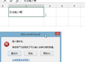
We use Microsoft Office Excel in various tasks such as processing data, tables, charts, etc., but when using Microsoft Office Excel, sometimes we will find that we cannot input content and prompt us that "the input value is illegal". Do you know how to cancel the limit on illegal input values in Excel? Let me demonstrate it to you. First, let's take a closer look at the high-definition pictures of the crime scene. When we enter content in cell C1, just press the Enter key and you will see the above prompt. 2. After canceling, return to the spreadsheet page and select cell C1. At this time, some people may find that there is a small drop-down triangle symbol in the lower right corner of cell C1, as shown in the picture. In fact, the problem is
