
 Computer Tutorials
Computer Knowledge
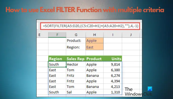
How to use Excel filter function with multiple conditions
Computer Tutorials
Computer Knowledge
How to use Excel filter function with multiple conditions
How to use Excel filter function with multiple conditions

If you need to know how to use the filter function with multiple conditions in Excel, the following tutorial will guide you through the corresponding steps to ensure that you can effectively filter and sort the data.
Excel’s filtering function is very powerful and can help you extract the information you need from large amounts of data. This function can filter data according to the conditions you set and display only the parts that meet the conditions, making data management more efficient. By using the filter function, you can quickly find target data, saving time in finding and organizing data. This function can not only be applied to simple data lists, but can also be filtered based on multiple conditions to help you locate the information you need more accurately. Overall, Excel's filtering function is a very practical tool that makes data analysis and processing more convenient.
What is the FILTER function in Excel?
The basic syntax for filtering data ranges, lists, or arrays using single or multiple conditions is as follows:
=筛选器(数组,包含,[IF_EMPTY])
So, if you want to extract specific data from a large amount of data, for example, from 1000 rows, this filter function formula makes the job easier. Previously, we only used dropdown lists with checkboxes to filter data, but this didn't help with complex conditions.
In other words, the Excel filter function has three input parameters:
- Array: The range of cells to be filtered.
- Includes: Criteria for filtering data that should be in the form of Boolean equations. For example, input using symbols such as =, >,
- [IF_EMPTY]: This optional input ("", N/A, or no results) instructs Excel to place a value or text string when the filter returns an empty table.
Basic formulas for using Excel filter functions
Before we explain how to use the Excel Filter function with multiple criteria, it is important to understand how the Excel Filter function formula works.
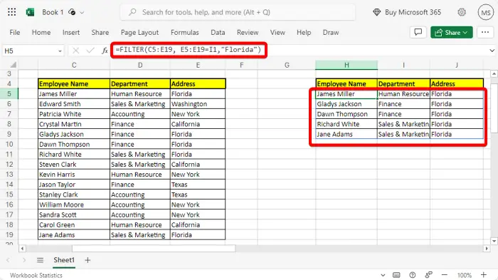
The following is an example of a basic Excel filter function formula, for example, filtering on the number of employees who stayed in Florida (see table):
=过滤器(C5:E19,E5:E19=I1,“佛罗里达”)
The formula extracts the results in the cell range (H4:J9) without changing the original data.
Alternatively, you can use the built-in filter functionality to make things easier. Just select the data range, go to the home page, and click the sort filter icon.
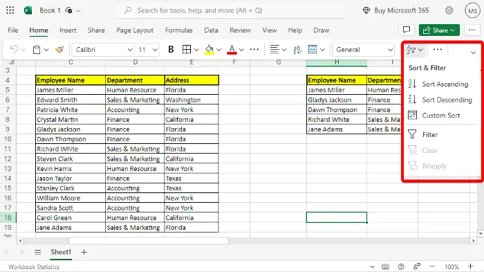
Select a filter from the menu to add a drop-down menu to the selected range.
Next, go to the Address column, select the dropdown, uncheck Select All, and select only Florida.
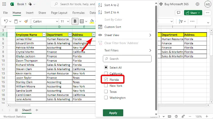
These cells now only display the names of Floridians and their respective departments.
However, if you encounter any SPILL errors in Excel, please refer to our linked post for solutions.
How to use Excel filter function under multiple conditions
Now that you know how to use basic filter functions in Excel, here is a Microsoft Excel tutorial on how to use filter functions with multiple conditions.
To use multiple conditions for data filtering, you can perform AND or OR operations.
1]Use AND operation with multiple conditions
The AND function requires all conditions to be True to include a row in the filtered results, while the OR function requires at least one condition to be True to include a row in the filtered results.
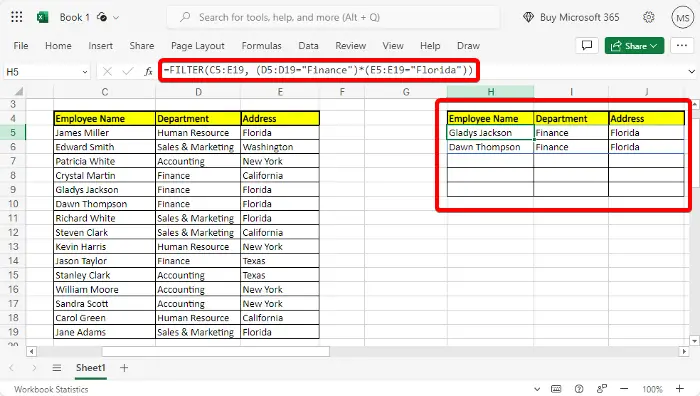
So, the following example illustrates how to use the AND logical function in Excel filter functions to extract data from a specific range of cells with two conditions:
=过滤器(C5:E19,(D5:D19=“金融”)*(E5:E19=“佛罗里达”))
This will extract how many finance department employees are from Florida.
Read: How to use slicers to filter data in Excel
2]Use OR operation with multiple conditions
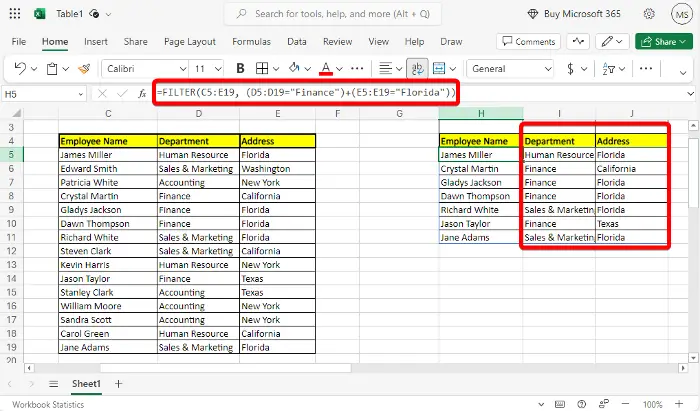
When any one or more conditions are met, the OR operation will be completed. So, for example, if you wanted to find out how many employees there are in the accounting department or the finance department, you would just use the formula above and replace the * operator with , like this:
=过滤器(C5:E19,(D5:D19=“金融”)+(E5:E19=“佛罗里达”))
就是这样,它应该在两个单独的列中返回两个结果。
但如果您更喜欢使用Microsoft Access,以下是如何在Access中对记录进行排序和筛选。
The above is the detailed content of How to use Excel filter function with multiple conditions. For more information, please follow other related articles on the PHP Chinese website!

Hot AI Tools

Undresser.AI Undress
AI-powered app for creating realistic nude photos

AI Clothes Remover
Online AI tool for removing clothes from photos.

Undress AI Tool
Undress images for free

Clothoff.io
AI clothes remover

Video Face Swap
Swap faces in any video effortlessly with our completely free AI face swap tool!

Hot Article
Hot Tools

Notepad++7.3.1
Easy-to-use and free code editor

SublimeText3 Chinese version
Chinese version, very easy to use

Zend Studio 13.0.1
Powerful PHP integrated development environment

Dreamweaver CS6
Visual web development tools

SublimeText3 Mac version
God-level code editing software (SublimeText3)
Hot Topics
 1387
1387
 52
52

 What should I do if the frame line disappears when printing in Excel?
Mar 21, 2024 am 09:50 AM
What should I do if the frame line disappears when printing in Excel?
Mar 21, 2024 am 09:50 AM
If when opening a file that needs to be printed, we will find that the table frame line has disappeared for some reason in the print preview. When encountering such a situation, we must deal with it in time. If this also appears in your print file If you have questions like this, then join the editor to learn the following course: What should I do if the frame line disappears when printing a table in Excel? 1. Open a file that needs to be printed, as shown in the figure below. 2. Select all required content areas, as shown in the figure below. 3. Right-click the mouse and select the "Format Cells" option, as shown in the figure below. 4. Click the “Border” option at the top of the window, as shown in the figure below. 5. Select the thin solid line pattern in the line style on the left, as shown in the figure below. 6. Select "Outer Border"
 How to filter more than 3 keywords at the same time in excel
Mar 21, 2024 pm 03:16 PM
How to filter more than 3 keywords at the same time in excel
Mar 21, 2024 pm 03:16 PM
Excel is often used to process data in daily office work, and it is often necessary to use the "filter" function. When we choose to perform "filtering" in Excel, we can only filter up to two conditions for the same column. So, do you know how to filter more than 3 keywords at the same time in Excel? Next, let me demonstrate it to you. The first method is to gradually add the conditions to the filter. If you want to filter out three qualifying details at the same time, you first need to filter out one of them step by step. At the beginning, you can first filter out employees with the surname "Wang" based on the conditions. Then click [OK], and then check [Add current selection to filter] in the filter results. The steps are as follows. Similarly, perform filtering separately again
 How to change excel table compatibility mode to normal mode
Mar 20, 2024 pm 08:01 PM
How to change excel table compatibility mode to normal mode
Mar 20, 2024 pm 08:01 PM
In our daily work and study, we copy Excel files from others, open them to add content or re-edit them, and then save them. Sometimes a compatibility check dialog box will appear, which is very troublesome. I don’t know Excel software. , can it be changed to normal mode? So below, the editor will bring you detailed steps to solve this problem, let us learn together. Finally, be sure to remember to save it. 1. Open a worksheet and display an additional compatibility mode in the name of the worksheet, as shown in the figure. 2. In this worksheet, after modifying the content and saving it, the dialog box of the compatibility checker always pops up. It is very troublesome to see this page, as shown in the figure. 3. Click the Office button, click Save As, and then
 Open source! Beyond ZoeDepth! DepthFM: Fast and accurate monocular depth estimation!
Apr 03, 2024 pm 12:04 PM
Open source! Beyond ZoeDepth! DepthFM: Fast and accurate monocular depth estimation!
Apr 03, 2024 pm 12:04 PM
0.What does this article do? We propose DepthFM: a versatile and fast state-of-the-art generative monocular depth estimation model. In addition to traditional depth estimation tasks, DepthFM also demonstrates state-of-the-art capabilities in downstream tasks such as depth inpainting. DepthFM is efficient and can synthesize depth maps within a few inference steps. Let’s read about this work together ~ 1. Paper information title: DepthFM: FastMonocularDepthEstimationwithFlowMatching Author: MingGui, JohannesS.Fischer, UlrichPrestel, PingchuanMa, Dmytr
 How to use the iif function in excel
Mar 20, 2024 pm 06:10 PM
How to use the iif function in excel
Mar 20, 2024 pm 06:10 PM
Most users use Excel to process table data. In fact, Excel also has a VBA program. Apart from experts, not many users have used this function. The iif function is often used when writing in VBA. It is actually the same as if The functions of the functions are similar. Let me introduce to you the usage of the iif function. There are iif functions in SQL statements and VBA code in Excel. The iif function is similar to the IF function in the excel worksheet. It performs true and false value judgment and returns different results based on the logically calculated true and false values. IF function usage is (condition, yes, no). IF statement and IIF function in VBA. The former IF statement is a control statement that can execute different statements according to conditions. The latter
 Where to set excel reading mode
Mar 21, 2024 am 08:40 AM
Where to set excel reading mode
Mar 21, 2024 am 08:40 AM
In the study of software, we are accustomed to using excel, not only because it is convenient, but also because it can meet a variety of formats needed in actual work, and excel is very flexible to use, and there is a mode that is convenient for reading. Today I brought For everyone: where to set the excel reading mode. 1. Turn on the computer, then open the Excel application and find the target data. 2. There are two ways to set the reading mode in Excel. The first one: In Excel, there are a large number of convenient processing methods distributed in the Excel layout. In the lower right corner of Excel, there is a shortcut to set the reading mode. Find the pattern of the cross mark and click it to enter the reading mode. There is a small three-dimensional mark on the right side of the cross mark.
 Google is ecstatic: JAX performance surpasses Pytorch and TensorFlow! It may become the fastest choice for GPU inference training
Apr 01, 2024 pm 07:46 PM
Google is ecstatic: JAX performance surpasses Pytorch and TensorFlow! It may become the fastest choice for GPU inference training
Apr 01, 2024 pm 07:46 PM
The performance of JAX, promoted by Google, has surpassed that of Pytorch and TensorFlow in recent benchmark tests, ranking first in 7 indicators. And the test was not done on the TPU with the best JAX performance. Although among developers, Pytorch is still more popular than Tensorflow. But in the future, perhaps more large models will be trained and run based on the JAX platform. Models Recently, the Keras team benchmarked three backends (TensorFlow, JAX, PyTorch) with the native PyTorch implementation and Keras2 with TensorFlow. First, they select a set of mainstream
 How to insert excel icons into PPT slides
Mar 26, 2024 pm 05:40 PM
How to insert excel icons into PPT slides
Mar 26, 2024 pm 05:40 PM
1. Open the PPT and turn the page to the page where you need to insert the excel icon. Click the Insert tab. 2. Click [Object]. 3. The following dialog box will pop up. 4. Click [Create from file] and click [Browse]. 5. Select the excel table to be inserted. 6. Click OK and the following page will pop up. 7. Check [Show as icon]. 8. Click OK.
