How to use the vlookup function-How to use the vlookup function

php editor Xiaoxin will give you an in-depth understanding of how to use the vlookup function. The vlookup function is a commonly used search function in Excel, which can help users find the location of specific values ​​in the table. Mastering the skills of using the vlookup function can improve the efficiency of data processing and make work more convenient. Flexible use of the vlookup function in Excel can easily achieve data search and matching, improving work efficiency. Want to know more detailed usage of vlookup function? Next, let’s dive into it!

1. Accurate search

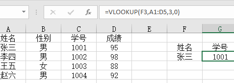
According to the precise information, query the corresponding data in the data table. In the figure, you can check the student ID by name, and use "=VLOOKUP(F3,A1:D5,4,0)".

2. Search with multiple conditions

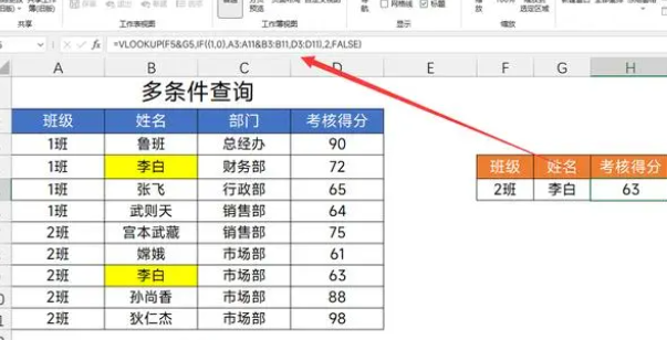
If there is duplicate data in the table, conditions must be added to limit the query. The formula used to find Class 2 Li Bai in the picture is "=VLOOKUP(F5&G5,IF({1,0},A3:A11&B3:B11,D3:D11),2,FALSE)".

3. Reverse search

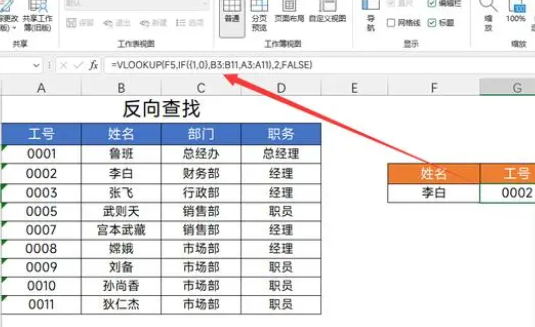
We want to use VLOOKUP to query Li Bai's job number, which is a reverse search. Find the job number on the left through the known name. The formula is "=VLOOKUP(F5,IF({1,0},B3:B11,A3: A11),2,FALSE)".

4. One-to-many query

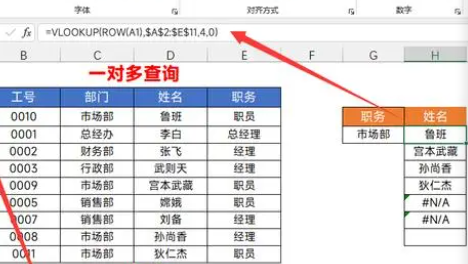
One piece of information matches multiple employees, and you can check the employee names by part. The picture takes the marketing department as an example to query the names of all employees in the marketing department. The formula is "=IFERROR(VLOOKUP(ROW(A1),$A$2:$E$11,4 ,0),"")".

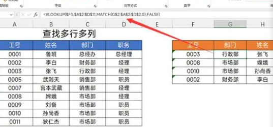
5. Automatically match the third parameter

Using one function, you can get multiple rows and columns of data. You can query the department and name through the employee number. The formula is "=VLOOKUP($F3,$A$2:$D$13,MATCH(H$2,$A$2:$ D$2,0),FALSE)”

6. Wildcard search

Wildcards are commonly used symbols

?: represents any 1 character

*: represents any number of characters

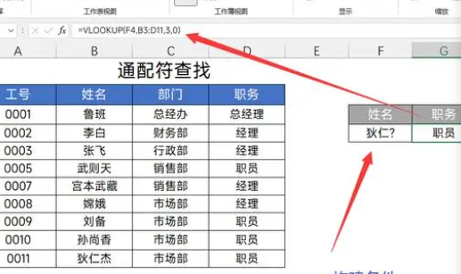
We can use wildcards to perform fuzzy searches. This is used when your information memory is fuzzy. If you don’t know the name, you can use this method to query. The formula in the picture is "=VLOOKUP(F4,B3:C11,2,0)".

7. Interval query

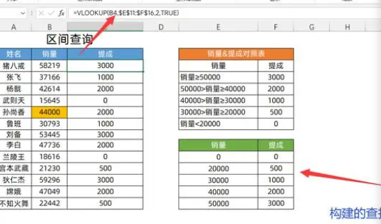
Interval query needs to build an interval first. The green marked data table in the figure is an interval. At this time, you can query the corresponding commission. However, please note that the fourth parameter is 1. The formula is "=VLOOKUP(B4,$E$11:$F$16 ,2,TRUE)”.

8. Data extraction

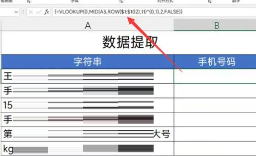
Obtain data from a bunch of characters, exclude non-numeric content, and identify valid information. The formula is "=VLOOKUP(0,MID(A3,ROW($1:$102),11)*{0,1},2,FALSE) ".

9. Find the maximum/nearest value

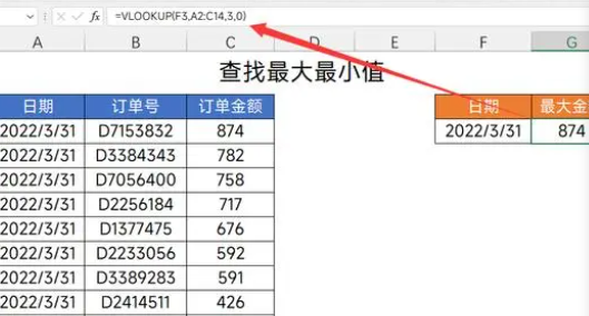
When looking for the maximum and minimum sales on a certain day, first use the "Sort" tool to "sort in descending order", and then use the formula "=VLOOKUP(F3,A2:C14,3,0)".

10. Skip empty character search

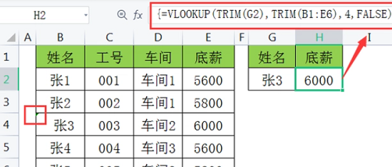
If there are spaces in the string, the result #N/A will be returned. In this case, you need to use the TRIM function to clear the spaces in the text, and then query the data. In the data table with spaces, query Zhang 3's basic salary. The formula is "=VLOOKUP(TRIM( G2),TRIM(B1:E6),4,FALSE)".

11. Merge cell query

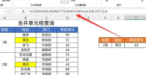
To merge data in different cells for query, you need to use the "INDIRECT" function to jump. The picture shows that when the name is known, the data is unified to query the results of Li Bai in class 2. The formula is "=VLOOKUP(G5,INDIRECT( "b"&MATCH(F5,A:A,0)&":D11"),3,0)".

The above is all the tutorials on how to use the vlookup function that the editor has brought to you. I hope it can be helpful to you.

The above is the detailed content of How to use the vlookup function-How to use the vlookup function. For more information, please follow other related articles on the PHP Chinese website!