Super strong! Top 10 deep learning algorithms!

Almost 20 years have passed since the concept of deep learning was proposed in 2006. As a revolution in the field of artificial intelligence, deep learning has spawned many influential algorithms. So, what do you think are the top 10 algorithms for deep learning?

The following are the top algorithms of deep learning in my mind. They all occupy an important position in terms of innovation, application value and influence.

1. Deep neural network (DNN)

Background: Deep neural network (DNN), also called multi-layer perceptron, is the most common The deep learning algorithm was criticized due to the bottleneck of computing power when it was first invented. It was not until the explosion of computing power and data in recent years that breakthroughs were made.

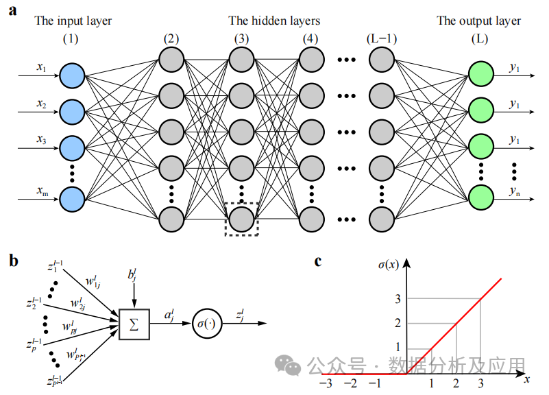
#DNN is a neural network model that contains multiple hidden layers. In this model, each layer passes input to the next layer and utilizes nonlinear activation functions to introduce nonlinear properties of learning. By superimposing these nonlinear transformations, DNN can learn complex feature representations of the input data.

Model training involves using the backpropagation algorithm and the gradient descent optimization algorithm to continuously adjust the weights. During training, the gradient of the loss function against the weights is calculated, and then gradient descent or other optimization algorithms are used to update the weights to minimize the loss function.

Advantages: Able to learn complex features of input data and capture non-linear relationships. It has powerful feature learning and representation capabilities.

Increasing network depth will lead to an increase in the vanishing gradient problem and unstable training. In addition, the model is prone to falling into local minima, requiring complex initialization strategies and regularization techniques.

Usage scenarios: image classification, speech recognition, natural language processing, recommendation system, etc.

Python sample code:

import numpy as npfrom keras.models import Sequentialfrom keras.layers import Dense# Assume there are 10 input features and 3 output categories input_dim = 10num_classes = 3# Create DNN model model = Sequential()model.add(Dense(64, activatinotallow='relu', input_shape=(input_dim,)))model.add(Dense(32, activatinotallow= 'relu'))model.add(Dense(num_classes, activatinotallow='softmax'))# Compile the model, select the optimizer and loss function model.compile(optimizer='adam', loss='categorical_crossentropy', metrics=[' accuracy'])# Assume there are 100 samples of training data and labels X_train = np.random.rand(100, input_dim)y_train = np.random.randint(0, 2, size=(100, num_classes))# Training model model.fit(X_train, y_train, epochs=10)

2. Convolutional Neural Network (CNN)

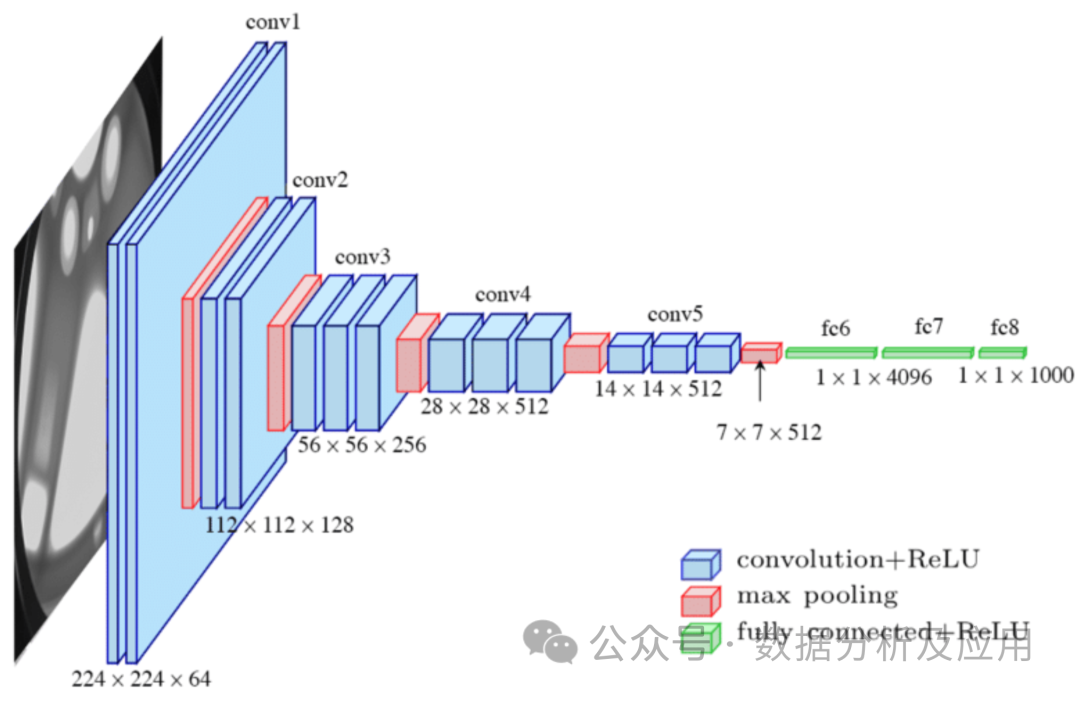
Model principle: Convolutional Neural Network (CNN) is a neural network specially designed for processing image data. , Lenet designed by Mr. Lechun is the pioneering work of CNN. CNN captures local features by using convolutional layers and reduces the dimensionality of the data through pooling layers. The convolutional layer performs a local convolution operation on the input data and uses a parameter sharing mechanism to reduce the number of parameters of the model. The pooling layer downsamples the output of the convolutional layer to reduce the dimensionality and computational complexity of the data. This structure is particularly suitable for processing image data.

Model training involves using the backpropagation algorithm and the gradient descent optimization algorithm to continuously adjust the weights. During training, the gradient of the loss function against the weights is calculated, and then gradient descent or other optimization algorithms are used to update the weights to minimize the loss function.

Advantages: Able to effectively process image data and capture local features. With a smaller number of parameters, the risk of overfitting is reduced.

Disadvantages: May not be suitable for sequence data or long-distance dependencies. Complex preprocessing of input data may be required.

Usage scenarios: image classification, target detection, semantic segmentation, etc.

Python example code

from keras.models import Sequentialfrom keras.layers import Conv2D, MaxPooling2D, Flatten, Dense# Assume the shape of the input image It is 64x64 pixels and has 3 color channels input_shape = (64, 64, 3)# Create CNN model model = Sequential()model.add(Conv2D(32, (3, 3), activatinotallow='relu', input_shape=input_shape ))model.add(MaxPooling2D((2, 2)))model.add(Conv2D(64, (3, 3), activatinotallow='relu'))model.add(Flatten())model.add(Dense( 128, activatinotallow='relu'))model.add(Dense(num_classes, activatinotallow='softmax'))# Compile the model, select the optimizer and loss function model.compile(optimizer='adam', loss='categorical_crossentropy', metrics=['accuracy'])# Assume there are 100 samples of training data and labels X_train = np.random.rand(100, *input_shape)y_train = np.random.randint(0, 2, size=(100, num_classes ))# Training model model.fit(X_train, y_train, epochs=10)

3. Residual Network (ResNet)

With the rapid development of deep learning, deep neural networks have achieved remarkable success in many fields. However, the training of deep neural networks faces problems such as gradient disappearance and model degradation, which limits the depth and performance of the network. In order to solve these problems, the residual network (ResNet) was proposed.

Model principle:

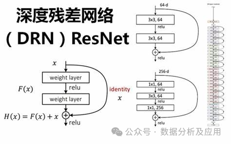
ResNet solves the problem of deep neural networks by introducing "residual blocks" vanishing gradient and model degradation problems. The residual block consists of a "skip connection" and one or more nonlinear layers, allowing gradients to be directly backpropagated from later layers to earlier layers, allowing for better training of deep neural networks. In this way, ResNet is able to build very deep network structures and achieve excellent performance on multiple tasks.

Model training:

The training of ResNet usually uses backpropagation algorithm and optimization algorithm (such as stochastic gradient descent). During the training process, the loss function is minimized by calculating the gradient of the loss function with respect to the weights and updating the weights using an optimization algorithm. In addition, in order to speed up the training process and improve the generalization ability of the model, regularization technology, ensemble learning and other methods can also be used.

Advantages:

1. # Solve the problem of gradient disappearance and model degradation: by introducing residual blocks and skip connections, ResNet can be more It can train deep neural networks well and avoid the problems of vanishing gradient and model degradation.
2. Build a very deep network structure: Due to solving the problems of gradient disappearance and model degradation, ResNet is able to build a very deep network structure, thus improving the performance of the model.
3. Achieved excellent performance on multiple tasks: Due to its powerful feature learning and representation capabilities, ResNet has achieved excellent performance on multiple tasks, such as image classification, target Testing etc.

Disadvantages:

1. Large amount of calculation: Since ResNet usually builds a very deep network structure, the amount of calculation is relatively large. Large, it requires higher computing resources and time for training.
2. Parameter tuning is difficult: ResNet has a large number of parameters, which requires a lot of time and energy for tuning and hyperparameter selection.
3. Sensitive to initialization weights: ResNet is highly sensitive to the selection of initialization weights. If the initialization weights are inappropriate, it may lead to unstable training or over-fitting problems.

Usage scenarios:

ResNet has a wide range of application scenarios in the field of computer vision, such as image classification, target detection, and face Recognition etc. In addition, ResNet can also be used in natural language processing, speech recognition and other fields.

Python sample code (simplified version):

In this simplified version of the example, we will demonstrate how to use the Keras library to build a simple ResNet model.

from keras.models import Sequentialfrom keras.layers import Conv2D, Add, Activation, BatchNormalization, Shortcutdef residual_block(input, filters):x = Conv2D(filters=filters, kernel_size=(3 , 3), padding='same')(input)x = BatchNormalization()(x)x = Activation('relu')(x)x = Conv2D(filters=filters, kernel_size=(3, 3), padding= 'same')(x)x = BatchNormalization()(x)x = Activation('relu')(x)return x

4. LSTM (Long Short-Term Memory Network)

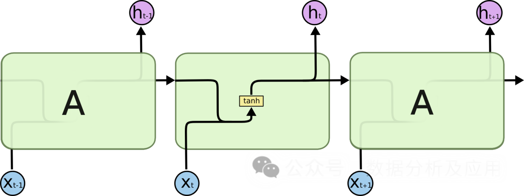
When processing sequence data, traditional recurrent neural networks (RNN) face problems such as gradient disappearance and model degradation. , which limits the depth and performance of the network. To solve these problems, LSTM was proposed.

Model principle:

LSTM controls the flow of information by introducing a "gating" mechanism. This solves the problems of gradient disappearance and model degradation. LSTM has three gating mechanisms: input gate, forget gate and output gate. The input gate determines the entry of new information, the forgetting gate determines the forgetting of old information, and the output gate determines the final output information. Through these gating mechanisms, LSTM is able to perform better on long-term dependency problems.

Model training:

The training of LSTM usually uses the back propagation algorithm and optimization algorithm (such as stochastic gradient descent). During the training process, the loss function is minimized by calculating the gradient of the loss function with respect to the weights and updating the weights using an optimization algorithm. In addition, in order to speed up the training process and improve the generalization ability of the model, regularization technology, ensemble learning and other methods can also be used.

Advantages:

1. # Solve the problem of gradient disappearance and model degradation: By introducing a gating mechanism, LSTM can better handle long-term Dependency problem avoids the problems of vanishing gradient and model degradation.
2. Build a very deep network structure: Due to solving the problems of gradient disappearance and model degradation, LSTM can build a very deep network structure, thus improving the performance of the model.
3. Achieved excellent performance on multiple tasks: Due to its powerful feature learning and representation capabilities, LSTM has achieved excellent performance on multiple tasks, such as text generation, speech Recognition, machine translation, etc.

Disadvantages:

1. Parameter tuning is difficult: LSTM has a large number of parameters, which requires a lot of time and energy Perform tuning and hyperparameter selection.
2. Sensitive to initialization weights: LSTM is highly sensitive to the selection of initialization weights. If the initialization weights are inappropriate, it may lead to unstable training or overfitting problems.
3. Large amount of calculation: Since LSTM usually builds a very deep network structure, it requires a large amount of calculation and requires high computing resources and time for training.

Usage scenarios:

LSTM has a wide range of application scenarios in the field of natural language processing, such as text generation, machine translation, speech Recognition etc. In addition, LSTM can also be used in fields such as time series analysis and recommendation systems.

Python sample code (simplified version):

from keras.models import Sequentialfrom keras.layers import LSTM, Densedef lstm_model(input_shape, num_classes ):model = Sequential()model.add(LSTM(units=128, input_shape=input_shape))# Add an LSTM layer model.add(Dense(units=num_classes, activatinotallow='softmax'))# Add a fully connected layer return model

5. Word2Vec

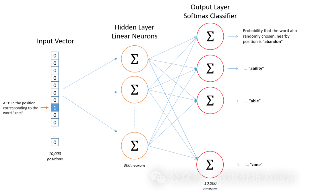
The Word2Vec model is the pioneering work of representation learning. A (shallow) neural network model for natural language processing developed by Google scientists. The goal of the Word2Vec model is to vectorize each word into a fixed-size vector so that similar words can be mapped to similar vector spaces.

Model Principle

The Word2Vec model is based on a neural network and uses the input word to predict its context words. During the training process, the model attempts to learn a vector representation of each word so that the word appearing in a given context is as close as possible to the vector representation of the target word. This training method is called "Skip-gram" or "Continuous Bag of Words" (CBOW).

Model training

Training the Word2Vec model requires a large amount of text data. First, the text data is preprocessed into a series of words or n-grams. Then, use a neural network to train the context of these words or n-grams. During the training process, the model continuously adjusts the vector representation of words to minimize prediction errors.

Advantages

1. Semantic similarity: Word2Vec can learn the semantic relationship between words, similar words in the vector The distance in space is similar.
2. Efficient training: The training process of Word2Vec is relatively efficient and can be trained on large-scale text data.
3. Interpretability: The word vector of Word2Vec has a certain degree of interpretability and can be used for tasks such as clustering, classification, and semantic similarity calculation.

Disadvantages

4. Data sparsity: Word2Vec may not be able to generate accurate vector representations for a large number of words that do not appear in the training data .
5. Context Window: Word2Vec only considers fixed-size contexts and may ignore further dependencies.
6. Computational Complexity: The training and inference process of Word2Vec requires a large amount of computing resources.
7. Parameter adjustment: The performance of Word2Vec is highly dependent on the settings of hyperparameters (such as vector dimensions, window size, learning rate, etc.).

Usage scenarios

Word2Vec is widely used in various natural language processing tasks, such as text classification, sentiment analysis, information extraction, etc. For example, Word2Vec can be used to identify the sentimental leanings (positive or negative) of news reports, or to extract key entities or concepts from large amounts of text.

Python sample code

from gensim.models import Word2Vecfrom nltk.tokenize import word_tokenizefrom nltk.corpus import abcimport nltk# Download and load abc corpus nltk.download ('abc')corpus = abc.sents()# Segment the corpus and convert it into lowercase sentences = [[word.lower() for word in word_tokenize(text)] for text in corpus]# Train the Word2Vec model model = Word2Vec( sentences, vector_size=100, window=5, min_count=5, workers=4)# Find the vector representation of the word "the" vector = model.wv['the']# Calculate the similarity with other words similarity = model.wv .similarity('the', 'of')# Print similarity value print(similarity)

6, Transformer

Background:

In the early stages of deep learning, convolutional neural networks (CNN) Remarkable successes have been achieved in the fields of image recognition and natural language processing. However, as task complexity increases, sequence-to-sequence (Seq2Seq) models and recurrent neural networks (RNN) become common methods for processing sequence data. Although RNN and its variants perform well on some tasks, they are prone to vanishing gradient and model degradation problems when processing long sequences. In order to solve these problems, the Transformer model was proposed. Later large models such as GPT and Bert were all based on Transformer to achieve excellent performance!

Model principle:

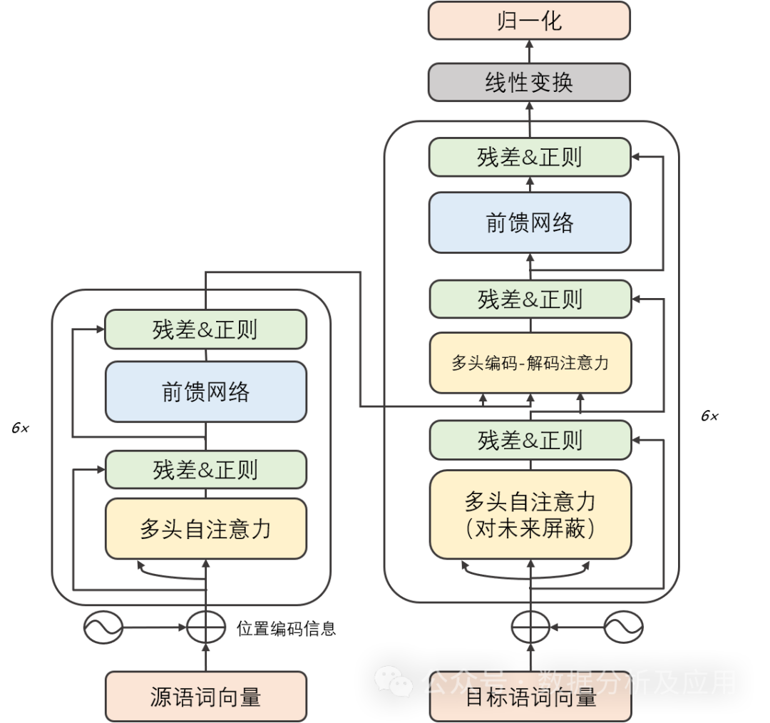
The Transformer model mainly consists of two parts: the encoder and the decoder. Each part is made up of multiple identical "layers". Each layer contains two sub-layers: self-attention sub-layer and linear feed-forward neural network sub-layer. The self-attention sub-layer uses the dot product attention mechanism to calculate the representation of each position in the input sequence, while the linear feed-forward neural network sub-layer takes the output of the self-attention layer as input and produces an output representation. Additionally, both the encoder and decoder contain a positional encoding layer to capture positional information in the input sequence.

Model training:

Transformer model training usually uses backpropagation algorithm and optimization algorithm (such as stochastic gradient descent). During the training process, the loss function is minimized by calculating the gradient of the loss function with respect to the weights and updating the weights using an optimization algorithm. In addition, in order to speed up the training process and improve the generalization ability of the model, regularization technology, ensemble learning and other methods can also be used.

Advantages:

1. # Solve the problem of gradient disappearance and model degradation: Since the Transformer model adopts the self-attention mechanism, it can be more It captures the long-term dependencies in the sequence well, thus avoiding the problems of vanishing gradient and model degradation.
2. Efficient parallel computing capabilities: Since the calculation of the Transformer model is parallelizable, training and inference can be performed quickly on the GPU.
3. Achieved excellent performance on multiple tasks: Due to its powerful feature learning and representation capabilities, the Transformer model has achieved excellent performance on multiple tasks, such as machine translation, Text classification, speech recognition, etc.

Disadvantages:

1. Large amount of calculation: Since the calculation of the Transformer model is parallelizable, it requires a large amount of Computing resources for training and inference.
2. Sensitive to initialization weights: The Transformer model is highly sensitive to the selection of initialization weights. If the initialization weights are inappropriate, it may lead to unstable training or overfitting problems.
3. Unable to learn long-term dependencies: Although the Transformer model solves the vanishing gradient and model degradation problems, there are still challenges when dealing with very long sequences.

Usage scenarios:

Transformer model has a wide range of application scenarios in the field of natural language processing, such as machine translation, text classification, Text generation, etc. In addition, the Transformer model can also be used in image recognition, speech recognition and other fields.

Python sample code (simplified version):

import torchimport torch.nn as nnimport torch.nn.functional as Fclass TransformerModel(nn.Module):def __init__(self, vocab_size, embedding_dim, num_heads, num_layers, dropout_rate=0.5):super(TransformerModel, self).__init__()self.embedding = nn.Embedding(vocab_size, embedding_dim)self.transformer = nn.Transformer(d_model=embedding_dim, nhead=num_heads, num_encoder_layers=num_layers, num_decoder_layers=num_layers, dropout=dropout_rate)self.fc = nn.Linear(embedding_dim, vocab_size)def forward(self, src, tgt):embedded = self.embedding(src)output = self.transformer(embedded)output = self.fc(output)return output pip install transformers

7. Generative Adversarial Network (GAN)

The idea of ​​GAN originates from the zero-sum game in game theory, in which one player tries to generate the most realistic fake data. While another player tries to distinguish real data from fake data. GAN evolved from the Monty Hall problem (a problem of combining a generative model and a discriminant model), but unlike the Monty Hall problem, GAN does not emphasize approximating certain probability distributions or generating certain samples, but directly uses Generative models versus discriminative models.

Model principle:

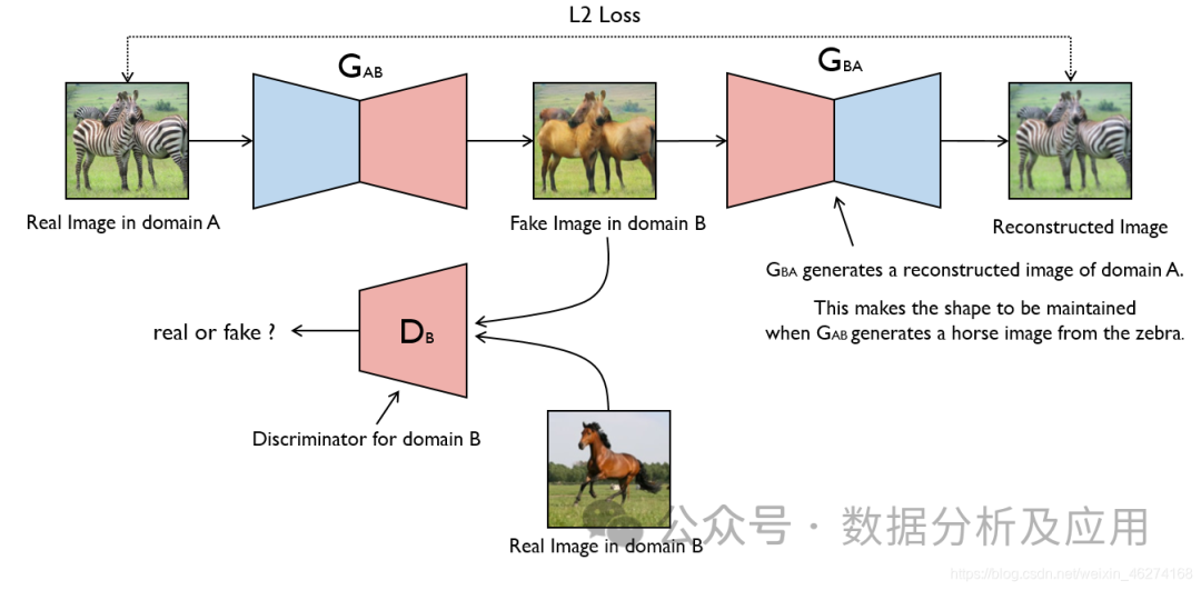
GAN consists of two parts: generator (Generator) and discriminator (Discriminator). The generator’s task is to generate fake data, while the discriminator’s task is to determine whether the input data comes from a real data set or fake data generated by the generator. During the training process, the generator and the discriminator compete, and parameters are constantly adjusted until an equilibrium state is reached. At this point, the fake data generated by the generator is realistic enough that the discriminator cannot distinguish real data from fake data.

Model training:

The training process of GAN is an optimization problem. In each training step, the generator under the current parameters is first used to generate fake data, and then the discriminator is used to determine whether the data is real or generated. Then, the parameters of the discriminator are updated based on this judgment result. At the same time, in order to prevent the discriminator from overfitting, the generator needs to be trained so that the generated fake data can deceive the discriminator. This process is repeated until an equilibrium state is reached.

Advantages:

1. Powerful generation ability: GAN can learn the intrinsic structure and distribution of data, thereby generating very realistic Fake data.
2. No explicit supervision required: No explicit label information is required during the training process of GAN, only real data is required.
3. High flexibility: GAN can be used in combination with other models, such as combining with autoencoders to form AutoGAN, or combining with convolutional neural networks to form DCGAN, etc.

Disadvantages:

1. Training is unstable: The training process of GAN is unstable and prone to mode collapse. ) problem, that is, the generator only generates a certain type of sample, causing the discriminator to be unable to judge correctly.
2. Difficult to debug: Debugging GANs is difficult because of the complex interactions between the generator and the discriminator.
3. Difficult to evaluate: Due to the strong generation ability of GAN, it is difficult to evaluate the authenticity and diversity of the fake data it generates.

Usage scenarios:

1. Image generation: GAN is most commonly used for image generation tasks and can generate various styles of Images, such as generating images based on text descriptions, converting one image to another style, etc.
2. Data enhancement: GAN can be used to generate fake data similar to real data to expand the data set or improve the generalization ability of the model.
3. Image repair: GAN can be used to repair defects in images or remove noise from images.
4. Video generation: GAN-based video generation is one of the hot spots in current research and can generate videos of various styles.

Simple Python sample code:

The following is a simple GAN sample code, implemented using PyTorch:

import torchimport torch.nn as nnimport torch.optim as optimimport torch.nn.functional as F# Define the generator and discriminator network structure class Generator(nn.Module):def __init__(self, input_dim, output_dim) :super(Generator, self).__init__()self.model = nn.Sequential(nn.Linear(input_dim, 128),nn.ReLU(),nn.Linear(128, output_dim),nn.Sigmoid())def forward(self, x):return self.model(x)class Discriminator(nn.Module):def __init__(self, input_dim):super(Discriminator, self).__init__()self.model = nn.Sequential(nn. Linear(input_dim, 128),nn.ReLU(),nn.Linear(128, 1),nn.Sigmoid())def forward(self, x):return self.model(x)# Instantiate generator and discriminator Generator object input_dim = 100# The input dimension can be adjusted according to actual needs output_dim = 784# For the MNIST data set, the output dimension is 28*28=784gen = Generator(input_dim, output_dim)disc = Discriminator(output_dim)# Define the loss function and optimizer criterion = nn.BCELoss()# The binary cross-entropy loss function is suitable for the discriminator part of GAN and the logistic loss part of the generator. However, a generally more common option is to employ a binary cross-entropy loss function (binary cross

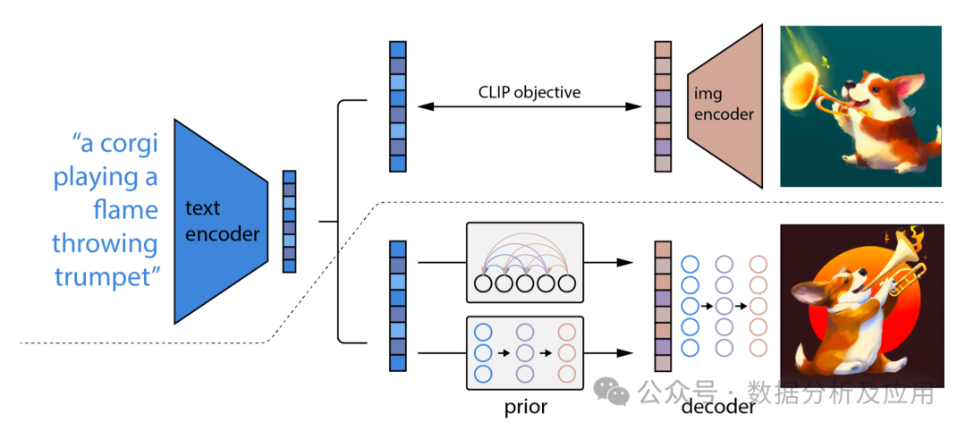
8. Diffusion diffusion model

The Diffusion model is a generative model based on deep learning. It is mainly used to generate continuous data, such as images, audio, etc. The core idea of ​​the Diffusion model is to convert complex data distribution into a simple Gaussian distribution by gradually adding noise, and then generating data from the simple distribution by gradually removing noise.

Model Principle

The Diffusion model contains two main processes: forward diffusion process and reverse diffusion process.

Forward diffusion process:

• Sample a data point (x_0) from the real data distribution.
• Within (T) time steps, gradually add noise to (x_0), generating a series of noise data points (x_1, x_2, ..., x_T) that gradually move away from the real data distribution.
• This process can be seen as gradually transforming the data distribution into a Gaussian distribution.

Reverse diffusion process (also called denoising process):

• Start from the noise data distribution (x_T), gradually remove the noise, and generate a series of data that is gradually closer to the real Data points of data distribution (x_{T-1}, x_{T-2}, ..., x_0).
• This process is to learn a neural network to predict the noise at each step, and use this prediction to gradually remove noise.

Model training

Training a Diffusion model usually involves the following steps:

1. Forward diffusion: For each sample (x_0) in the training data set, According to the predetermined noise scheduling plan, the corresponding noise sequence (x_1, x_2, ..., x_T) is generated.
2. Noise prediction: For each time step (t), train a neural network to predict the noise in (x_t). This neural network is usually a conditional variational autoencoder (CVAE), which receives (x_t) and time step (t) as input and outputs predicted noise.
3. Optimization: Optimize neural network parameters by minimizing the difference between real noise and predicted noise. A commonly used loss function is Mean Squared Error (MSE).

Advantages

• Powerful generation capabilities: The Diffusion model can generate high-quality, diverse data samples.
• Progressive generation: The model can provide intermediate results during the generation process, which helps to understand the model generation process.
• Stable training: Compared with some other generative models (such as GANs), diffusion models are generally easier to train and less prone to mode collapse problems.

Disadvantages

• Computationally intensive: Due to the need for forward and reverse diffusion over multiple time steps, the training and generation process of the Diffusion model is usually time-consuming .
• High number of parameters: For each time step, a separate neural network is required for noise prediction, which results in a large number of model parameters.

Usage scenarios

The Diffusion model is suitable for scenarios where continuous data needs to be generated, such as image generation, audio generation, video generation, etc. In addition, because the model has the characteristics of progressive generation, it can also be used for tasks such as data interpolation and style transfer.

Python sample code

The following is a simplified sample code for Diffusion model training, using the PyTorch library:

import torchimport torch.nn as nnimport torch.optim as optim# Suppose we have a simple Diffusion model class DiffusionModel(nn.Module):def __init__(self, input_dim, hidden_dim, num_timesteps):super(DiffusionModel , self).__init__()self.num_timesteps = num_timestepsself.noises = nn.ModuleList([nn.Linear(input_dim, hidden_dim),nn.ReLU(),nn.Linear(hidden_dim, input_dim)] for _ in range(num_timesteps ))def forward(self, x, t):noise_prediction = self.noises[t](x)return noise_prediction# Set the model parameter input_dim = 784# Assume that the input is a 28x28 grayscale image hidden_dim = 128num_timesteps = 1000# Initialize the model model = DiffusionModel(input_dim, hidden_dim, num_timesteps)# Define the loss function and optimizer criterion = nn.MSELoss()optimizer = optim.Adam(model.parameters(), lr=1e-3)

9. Graph Neural Network (GNN)

Graph Neural Networks (GNN for short) is a deep learning model specially used to process graph-structured data. In the real world, many complex systems can be represented by graphs, such as social networks, molecular structures, transportation networks, etc. Traditional machine learning models face many challenges when processing these graph-structured data, and graph neural networks provide new ideas for solving these problems.

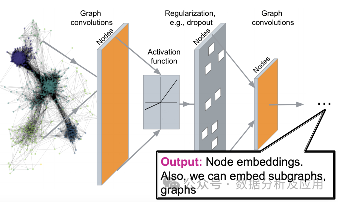
Model principle:

The core idea of ​​graph neural network is to learn feature representation of nodes in the graph through neural network, while taking into account the relationship between nodes . Specifically, GNN updates the representation of nodes by iteratively transferring neighbor information, so that nodes in the same community or close have similar representations. At each layer, a node updates its representation based on information about its neighbor nodes, thereby capturing complex patterns in the graph.

Model training:

Training graph neural networks usually uses gradient-based optimization algorithms, such as stochastic gradient descent (SGD). During the training process, the gradient of the loss function is calculated through the backpropagation algorithm and the weights of the neural network are updated. Commonly used loss functions include cross-entropy loss for node classification, binary cross-entropy loss for link prediction, etc.

Advantages:

• Powerful representation ability: Graph neural network can effectively capture complex patterns in graph structures, thereby achieving better results in tasks such as node classification and link prediction. Effect.
• Natural processing of graph-structured data: Graph neural networks directly process graph-structured data without converting the graph into matrix form, thereby avoiding the computing and storage overhead caused by large-scale sparse matrices.
• Strong scalability: Graph neural networks can capture more complex patterns by stacking more layers and are highly scalable.

Disadvantages:

• High computational complexity: As the number of nodes and edges in the graph increases, the computational complexity of the graph neural network will also increase sharply, which may lead to Training time is longer.
• Difficulty in parameter adjustment: Graph neural networks have many hyperparameters, such as neighborhood size, number of layers, learning rate, etc. Adjusting these parameters may require an in-depth understanding of the task.
• Different adaptability to undirected graphs and directed graphs: Graph neural networks were originally designed for undirected graphs, and may have poor adaptability to directed graphs.

Usage scenarios:

• Social network analysis: In social networks, the relationships between users can be represented by graphs. Graph neural networks can analyze issues such as similarities between users, community discovery, and influence dissemination.
• Molecular structure prediction: In the field of chemistry, the structure of a molecule can be represented by a diagram. By training graph neural networks, the properties of molecules, chemical reactions, etc. can be predicted.
• Recommendation system: The recommendation system can use the user's behavioral data to construct a graph, and then use the graph neural network to capture the user's behavior pattern to make accurate recommendations.
• Knowledge graph: Knowledge graph can be regarded as a special graph structure data. The entities and relationships in the knowledge graph can be deeply analyzed through graph neural network.

Simple Python example code:

import torchfrom torch_geometric.datasets import Planetoidfrom torch_geometric.nn import GCNConvfrom torch_geometric.data import DataLoaderimport time# Load Cora dataset dataset = Planetoid(root='/tmp/Cora', name='Cora')# Definition GNN model class GNN(torch.nn.Module):def __init__(self, in_channels, hidden_channels, out_channels):super(GNN, self).__init__()self.conv1 = GCNConv(in_channels, hidden_channels)self.conv2 = GCNConv( hidden_channels, out_channels)def forward(self, data):x, edge_index = data.x, data.edge_indexx = self.conv1(x, edge_index)x = F.relu(x)x = F.dropout(x, training= self.training)x = self.conv2(x, edge_index)return F.log_softmax(x, dim=1)# Define hyperparameters and model training process num_epochs = 1000lr = 0.01hidden_channels = 16out_channels = dataset.num_classesdata = dataset[0] # Use the first data in the dataset as example data model = GNN(dataset.num_features, hidden_channels, out_channels)optimizer = torch.optim.Adam(model.parameters(), lr=lr)data = DataLoader([data], batch_size=1)# Convert the data set into a DataLoader object to support batch training and evaluation model.train()# Set the model to training mode for epoch in range(num_epochs):for data in data:# Traverse in each epoch The entire data set is optimized once optimizer.zero_grad()# Clear the gradient out = model(data)# Forward propagation, calculate the output and loss function value loss = F.nll_loss(out[data.train_mask], data.y[data.train_mask ])# Calculate the loss function value, here we use the negative log-likelihood loss function as an example loss function loss.backward()# Backward propagation, calculate the gradient optimizer.step()# Update the weight parameters

10. Deep Q Network (DQN)

In traditional reinforcement learning algorithms, agents use a Q table to store estimates of the state-action value function. However, this approach encounters limitations when dealing with high-dimensional state and action spaces. In order to solve this problem, DQN is a deep reinforcement learning algorithm that introduces deep learning technology to learn the approximation of the state-action value function, so that it can handle more complex problems.

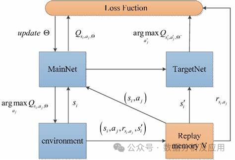
Model principle:

DQN uses a neural network (called a deep Q network) to approximate the state-action value function. This neural network accepts the current state as input and outputs a Q-value for each action. During the training process, the agent updates the weights of the neural network by constantly interacting with the environment to gradually approach the optimal Q-value function.

Model training:

The training process of DQN includes two stages: offline stage and online stage. In the offline phase, the agent randomly samples a batch of experiences (i.e., states, actions, rewards, and next states) from the experience replay buffer and uses these experiences to update the deep Q network. In the online phase, the agent uses the current state and the deep Q network to select and execute the best action, and stores new experiences in the experience replay buffer.

Advantages:

• Processing high-dimensional state and action spaces: DQN is able to handle complex problems with high-dimensional state and action spaces, which makes it widely used in many fields. .
• Reduce data dependence: By using the experience replay buffer, DQN can be trained effectively with limited samples.
• Flexibility: DQN can be combined with other reinforcement learning algorithms and techniques to further improve performance and expand its application scope.

Disadvantages:

• Unstable training: In some cases, the training of DQN may be unstable, causing the learning process to fail or performance to degrade.
• Exploration strategy: DQN requires an effective exploration strategy to explore the environment and collect enough experience. Choosing an appropriate exploration strategy is key as it can affect learning speed and final performance.
• Requirement for target network: In order to stabilize training, DQN usually needs to use the target network to update the Q-value function. This increases the complexity of the algorithm and requires additional parameter tuning.

Usage scenarios:

DQN has been widely used in various game AI tasks, such as Go, card games, etc. In addition, it is also used in other fields such as robot control, natural language processing and autonomous driving.

pythonimport numpy as npimport tensorflow as tffrom tensorflow.keras.models import Sequentialfrom tensorflow.keras.layers import Dense, Dropoutclass DQN:def __init__(self, state_size, action_size):self.state_size = state_sizeself.action_size = action_sizeself.memory = np.zeros((MEM_CAPACITY, state_size * 2   2))self.gamma = 0.95self.epsilon = 1.0self.epsilon_min = 0.01self.epsilon_decay = 0.995self.learning_rate = 0.005self.model = self.create_model()def create_model(self):model = Sequential()model.add(Dense(24, input_dim=self.state_size, activation='relu'))model.add(Dense(24, activation='relu'))model.add(Dense(self.action_size, activation='linear'))model.compile(loss='mse', optimizer=tf.keras.optimizers.Adam(lr=self.learning_rate))return modeldef remember(self, state, action, reward, next_state, done):self.memory[self.memory_counter % MEM_CAPACITY, :] = [state, action, reward, next_state, done]self.memory_counter  = 1def act(self, state):if np.random.rand() 

The above is the detailed content of Super strong! Top 10 deep learning algorithms!. For more information, please follow other related articles on the PHP Chinese website!