 Technology peripherals
 AI
AI
 With only 200M parameters, zero-sample performance surpasses supervised! Google releases basic time series prediction model TimesFM
With only 200M parameters, zero-sample performance surpasses supervised! Google releases basic time series prediction model TimesFM
Time series forecasting plays an important role in various fields, such as retail, finance, manufacturing, healthcare, and natural sciences, etc. In the retail industry, inventory costs can be effectively reduced and revenue increased by improving the accuracy of demand forecasts. This means businesses can better meet customer demand, reduce inventory overhang and losses, while increasing sales and profits. Therefore, time series forecasting is of great value in the retail field and can bring substantial benefits to enterprises
Deep learning (DL) models dominate the task of "multivariable time series forecasting" status, showing excellent performance in various competitions and practical applications.
At the same time, significant progress has been made in large-scale basic language models in natural language processing (NLP) tasks, effectively improving tasks such as translation, retrieval enhancement generation, and code completion. performance.
The training of NLP models relies on massive text data, which comes from a variety of sources, including crawlers, open source code, etc. The trained model can recognize patterns in the language and has zero The ability of sample learning: For example, when using a large model for retrieval tasks, the model can answer questions about current events and summarize them.
Although deep learning-based predictors outperform traditional methods in many ways, including reducing training and inference costs, there are still some challenges that need to be overcome:
Many deep learning models undergo lengthy training and validation before they can be tested on new time series. In contrast, the underlying model for time series forecasting has "out-of-the-box forecasting" capabilities and can be applied to unknown time series data without additional training. This feature allows users to focus on improving forecasting for practical downstream tasks such as retail demand planning.
Researchers at Google Research recently proposed a basic model for time series prediction called TimesFM, which was pre-trained on 100 billion real-world time points. Compared with current state-of-the-art large language models (LLMs), TimesFM is much smaller in size, containing only 200M parameters.

Paper link: https://arxiv.org/pdf/2310.10688.pdf
Experiment The results show that despite its small size, TimesFM exhibits surprising "zero-shot performance" on different untrained datasets across various domains and time scales, approaching the performance of unambiguously trained, state-of-the-art supervised methods on these performance on the data set.
The researchers plan to make the TimesFM model available to external customers in Google Cloud Vertex AI later this year.
Basic model TimesFM
LLMs are usually trained in a decoder-only manner, including three steps:
1. Text is broken down into subwords called tokens
2. Tokens are fed into stacked causal Transformer layers and generated with each input token Corresponding output, it should be noted that this layer cannot handle tokens without input, that is, future tokens
3. The output corresponding to the i-th token summarizes all the information from the previous tokens. information, and predict the (i 1)th token
During inference, LLM generates the output of one token at a time.
For example, when inputting the prompt "What is the capital of France?" (What is the capital of France?), the model may generate the token "The", and then use this prompt Generate the next token "capital" for the condition, and so on, until the model generates a complete answer: "The capital of France is Paris" (The capital of France is Paris).
The underlying model for time series forecasting should adapt to variable context (what the model observes) and range (what the query model predicts) lengths, while having sufficient power to encode data from large pre-trained datasets. All patterns.
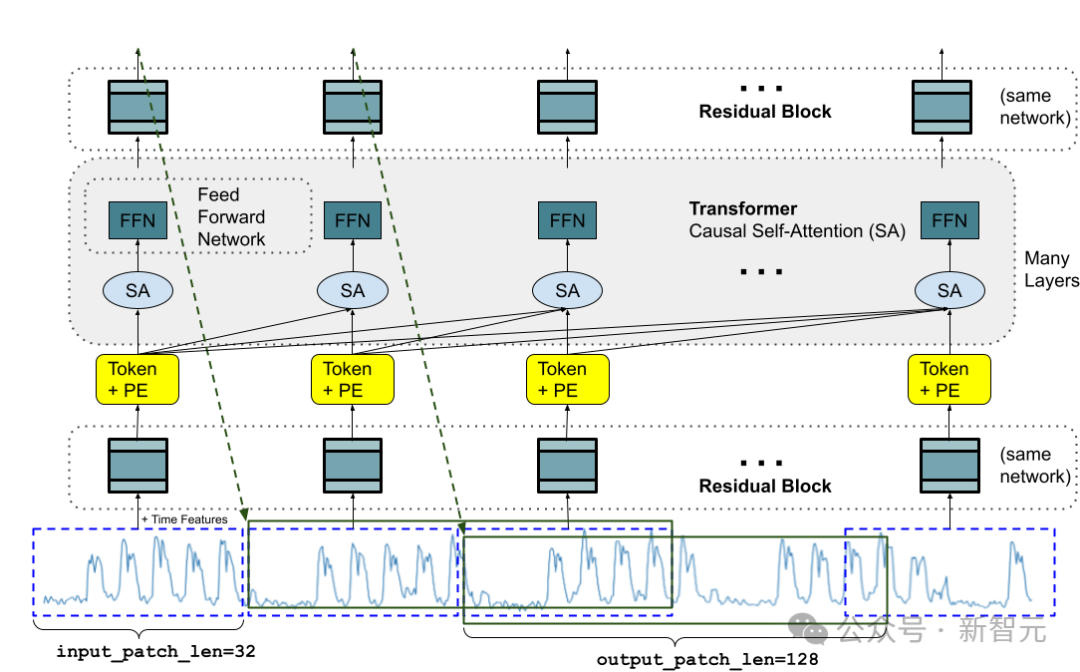
Similar to LLMs, the researchers used stacked Transformer layers (self-attention and feed-forward layers) as the main building blocks of the TimesFM model; in In the context of time series forecasting, a patch (a set of consecutive time points) is used as a token. The idea comes from recent long-horizon forecasting work: the specific task is to predict at the end of the stacked Transformer layer, for a given th i output to predict the (i 1)th time point patch
But TimesFM has several key differences with the language model:
1. The model requires a multi-layer perceptron block with residual connections to convert the time series patches into tokens, which can be input to the Transformer layer along with the position encoding (PE). To do this, we use residual blocks similar to our previous work in long-term prediction.
2. The output token from the stacked Transformer can be used to predict the length of subsequent time points that is longer than the input patch length, that is, the output patch length can be greater than the input patch length.
Assume that a time series with a length of 512 time points is used to train a TimesFM model with "input patch length 32" and "output patch length 128":
During training, the model is simultaneously trained to use the first 32 time points to predict the next 128 time points, the first 64 time points to predict time points 65 to 192, and the first 96 time points to predict time points 97 to 224 and so on.
Assuming that the input data is a time series of length 256, and its task is to predict the next 256 time points in the future, the model first generates future predictions for time points 257 to 384, Time points 385 to 512 are then generated conditioned on the initial 256 length input plus the generated output.
On the other hand, if in the model, the output patch length is equal to the input patch length 32, then for the same task, the model goes through eight generation steps instead of 2, increasing the error Cumulative risk, so it can be seen in the experimental results that longer output patch length leads to better long-term prediction performance.
Pre-training data
Just like LLMs can get better with more tokens, TimesFM requires a large amount of legitimate time series data to learn and improve; researchers After spending a lot of time creating and evaluating training data sets, I found two better methods:
Synthetic data helps with the basics
Meaningful synthetic time series data can be generated using statistical models or physical simulations, and basic temporal patterns can guide the model to learn the syntax of time series forecasting.
Real-world data adds real-world flavor
The researchers combed through available public time series datasets and selectively put together a large corpus of 100 billion time points.
In the data set, there are Google Trends and Wikipedia page views, which track what users are interested in, and reflect well the trends and patterns of many other real-world time series , helps TimesFM understand the bigger picture, and can improve generalization performance for "domain-specific contexts that have not been seen during training."
Zero-sample evaluation results
The researchers used a commonly used time series benchmark to conduct a zero-sample evaluation of TimesFM on data not seen during training, and it was observed that TimesFM performed better than most Statistical methods such as ARIMA, ETS, and can match or outperform powerful DL models such as DeepAR, PatchTST that have been explicitly trained on the target time series.
The researchers used the Monash Forecasting Archive to evaluate the out-of-box performance of TimesFM, a dataset containing tens of thousands of time series from various domains such as traffic, weather and demand forecasting, Coverage frequency ranges from a few minutes to yearly data.
Based on existing literature, the researchers examined the mean absolute error (MAE) appropriately scaled to average over the data set.
As can be seen, zero-shot (ZS) TimesFM outperforms most supervised methods, including recent deep learning models. TimesFM and GPT-3.5 were also compared for prediction using the specific hint technology proposed by llmtime (ZS), and the results proved that TimesFM performed better than llmtime (ZS)
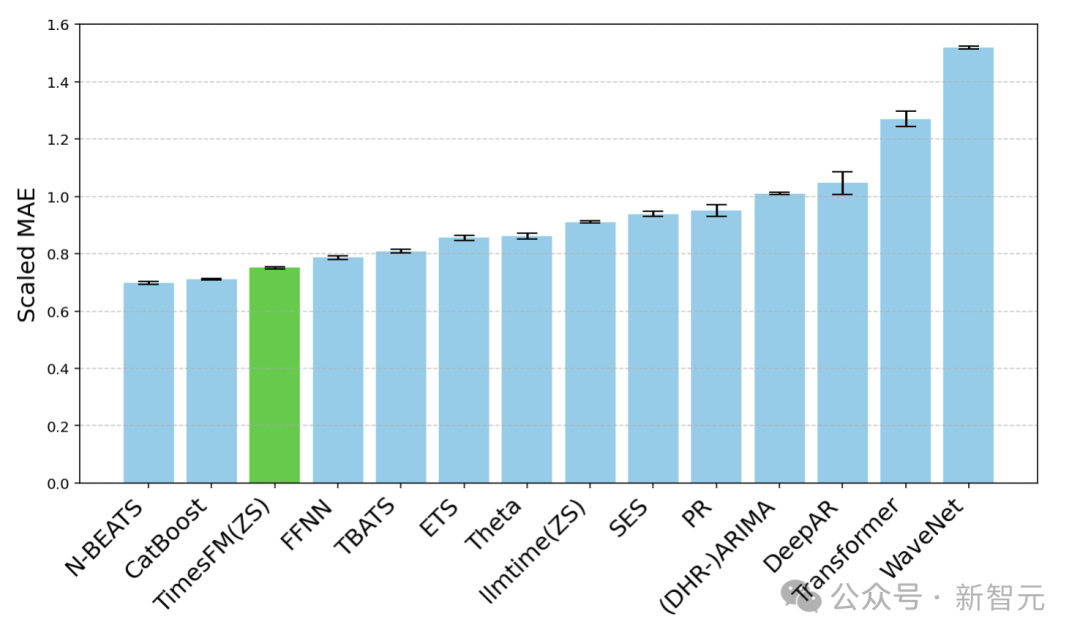
Ratio MAE of TimesFM (ZS) vs. other supervised and zero-shot methods on Monash dataset (lower is better)
Most Monash datasets are Short or medium-term, meaning the forecast length is not too long; the researchers also tested TimesFM against a commonly used benchmark long-term forecast against the state-of-the-art baseline PatchTST (and other long-term forecast baselines).
The researchers plotted the MAE on the ETT dataset for the task of predicting 96 and 192 time points into the future, calculating the metric on the last test window of each dataset.
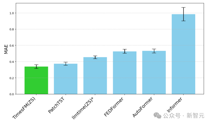
Last window MAE (lower is better) of TimesFM(ZS) versus llmtime(ZS) and long-term forecast on ETT dataset Baseline
It can be seen that TimesFM not only exceeds the performance of llmtime (ZS), but also matches the performance of the supervised PatchTST model explicitly trained on the corresponding dataset.
Conclusion
The researchers trained a base decoder-only model using a large pre-training corpus of 100 billion real-world time points, most of which were Search interest time series data from Google Trends and Wikipedia page views.
The results show that even a relatively small 200 M parameter pre-trained model, using the TimesFM architecture, exhibits excellent performance in various public benchmarks (different domains and granularities) Pretty good zero-shot performance.
The above is the detailed content of With only 200M parameters, zero-sample performance surpasses supervised! Google releases basic time series prediction model TimesFM. For more information, please follow other related articles on the PHP Chinese website!

Hot AI Tools

Undresser.AI Undress
AI-powered app for creating realistic nude photos

AI Clothes Remover
Online AI tool for removing clothes from photos.

Undress AI Tool
Undress images for free

Clothoff.io
AI clothes remover

AI Hentai Generator
Generate AI Hentai for free.

Hot Article

Hot Tools

Notepad++7.3.1
Easy-to-use and free code editor

SublimeText3 Chinese version
Chinese version, very easy to use

Zend Studio 13.0.1
Powerful PHP integrated development environment

Dreamweaver CS6
Visual web development tools

SublimeText3 Mac version
God-level code editing software (SublimeText3)

Hot Topics
 Open source! Beyond ZoeDepth! DepthFM: Fast and accurate monocular depth estimation!
Apr 03, 2024 pm 12:04 PM
0.What does this article do? We propose DepthFM: a versatile and fast state-of-the-art generative monocular depth estimation model. In addition to traditional depth estimation tasks, DepthFM also demonstrates state-of-the-art capabilities in downstream tasks such as depth inpainting. DepthFM is efficient and can synthesize depth maps within a few inference steps. Let’s read about this work together ~ 1. Paper information title: DepthFM: FastMonocularDepthEstimationwithFlowMatching Author: MingGui, JohannesS.Fischer, UlrichPrestel, PingchuanMa, Dmytr
 The world's most powerful open source MoE model is here, with Chinese capabilities comparable to GPT-4, and the price is only nearly one percent of GPT-4-Turbo
May 07, 2024 pm 04:13 PM
Imagine an artificial intelligence model that not only has the ability to surpass traditional computing, but also achieves more efficient performance at a lower cost. This is not science fiction, DeepSeek-V2[1], the world’s most powerful open source MoE model is here. DeepSeek-V2 is a powerful mixture of experts (MoE) language model with the characteristics of economical training and efficient inference. It consists of 236B parameters, 21B of which are used to activate each marker. Compared with DeepSeek67B, DeepSeek-V2 has stronger performance, while saving 42.5% of training costs, reducing KV cache by 93.3%, and increasing the maximum generation throughput to 5.76 times. DeepSeek is a company exploring general artificial intelligence
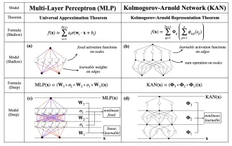 KAN, which replaces MLP, has been extended to convolution by open source projects
Jun 01, 2024 pm 10:03 PM
Earlier this month, researchers from MIT and other institutions proposed a very promising alternative to MLP - KAN. KAN outperforms MLP in terms of accuracy and interpretability. And it can outperform MLP running with a larger number of parameters with a very small number of parameters. For example, the authors stated that they used KAN to reproduce DeepMind's results with a smaller network and a higher degree of automation. Specifically, DeepMind's MLP has about 300,000 parameters, while KAN only has about 200 parameters. KAN has a strong mathematical foundation like MLP. MLP is based on the universal approximation theorem, while KAN is based on the Kolmogorov-Arnold representation theorem. As shown in the figure below, KAN has
 Hello, electric Atlas! Boston Dynamics robot comes back to life, 180-degree weird moves scare Musk
Apr 18, 2024 pm 07:58 PM
Boston Dynamics Atlas officially enters the era of electric robots! Yesterday, the hydraulic Atlas just "tearfully" withdrew from the stage of history. Today, Boston Dynamics announced that the electric Atlas is on the job. It seems that in the field of commercial humanoid robots, Boston Dynamics is determined to compete with Tesla. After the new video was released, it had already been viewed by more than one million people in just ten hours. The old people leave and new roles appear. This is a historical necessity. There is no doubt that this year is the explosive year of humanoid robots. Netizens commented: The advancement of robots has made this year's opening ceremony look like a human, and the degree of freedom is far greater than that of humans. But is this really not a horror movie? At the beginning of the video, Atlas is lying calmly on the ground, seemingly on his back. What follows is jaw-dropping
 AI subverts mathematical research! Fields Medal winner and Chinese-American mathematician led 11 top-ranked papers | Liked by Terence Tao
Apr 09, 2024 am 11:52 AM
AI is indeed changing mathematics. Recently, Tao Zhexuan, who has been paying close attention to this issue, forwarded the latest issue of "Bulletin of the American Mathematical Society" (Bulletin of the American Mathematical Society). Focusing on the topic "Will machines change mathematics?", many mathematicians expressed their opinions. The whole process was full of sparks, hardcore and exciting. The author has a strong lineup, including Fields Medal winner Akshay Venkatesh, Chinese mathematician Zheng Lejun, NYU computer scientist Ernest Davis and many other well-known scholars in the industry. The world of AI has changed dramatically. You know, many of these articles were submitted a year ago.
 The vitality of super intelligence awakens! But with the arrival of self-updating AI, mothers no longer have to worry about data bottlenecks
Apr 29, 2024 pm 06:55 PM
I cry to death. The world is madly building big models. The data on the Internet is not enough. It is not enough at all. The training model looks like "The Hunger Games", and AI researchers around the world are worrying about how to feed these data voracious eaters. This problem is particularly prominent in multi-modal tasks. At a time when nothing could be done, a start-up team from the Department of Renmin University of China used its own new model to become the first in China to make "model-generated data feed itself" a reality. Moreover, it is a two-pronged approach on the understanding side and the generation side. Both sides can generate high-quality, multi-modal new data and provide data feedback to the model itself. What is a model? Awaker 1.0, a large multi-modal model that just appeared on the Zhongguancun Forum. Who is the team? Sophon engine. Founded by Gao Yizhao, a doctoral student at Renmin University’s Hillhouse School of Artificial Intelligence.
 Kuaishou version of Sora 'Ke Ling' is open for testing: generates over 120s video, understands physics better, and can accurately model complex movements
Jun 11, 2024 am 09:51 AM
What? Is Zootopia brought into reality by domestic AI? Exposed together with the video is a new large-scale domestic video generation model called "Keling". Sora uses a similar technical route and combines a number of self-developed technological innovations to produce videos that not only have large and reasonable movements, but also simulate the characteristics of the physical world and have strong conceptual combination capabilities and imagination. According to the data, Keling supports the generation of ultra-long videos of up to 2 minutes at 30fps, with resolutions up to 1080p, and supports multiple aspect ratios. Another important point is that Keling is not a demo or video result demonstration released by the laboratory, but a product-level application launched by Kuaishou, a leading player in the short video field. Moreover, the main focus is to be pragmatic, not to write blank checks, and to go online as soon as it is released. The large model of Ke Ling is already available in Kuaiying.
 The U.S. Air Force showcases its first AI fighter jet with high profile! The minister personally conducted the test drive without interfering during the whole process, and 100,000 lines of code were tested for 21 times.
May 07, 2024 pm 05:00 PM
Recently, the military circle has been overwhelmed by the news: US military fighter jets can now complete fully automatic air combat using AI. Yes, just recently, the US military’s AI fighter jet was made public for the first time and the mystery was unveiled. The full name of this fighter is the Variable Stability Simulator Test Aircraft (VISTA). It was personally flown by the Secretary of the US Air Force to simulate a one-on-one air battle. On May 2, U.S. Air Force Secretary Frank Kendall took off in an X-62AVISTA at Edwards Air Force Base. Note that during the one-hour flight, all flight actions were completed autonomously by AI! Kendall said - "For the past few decades, we have been thinking about the unlimited potential of autonomous air-to-air combat, but it has always seemed out of reach." However now,


