Basic tutorial on using excel

php editor Banana brings you a basic tutorial on how to use Excel. As a commonly used office software, Excel has powerful data processing and analysis functions. This tutorial will introduce in detail the basic operations, formula application, data filtering, etc. of Excel to help you quickly master the skills of using Excel. Whether you are a beginner or a user who wants to improve your skills, you can gain practical knowledge from this tutorial and improve your work efficiency. Let’s explore the mysteries of Excel together!

1. Set the column width and row height

Select the entire row or column of cells, right-click the mouse and select "Column Width" or "Row Height", fill in the set value, and you are done

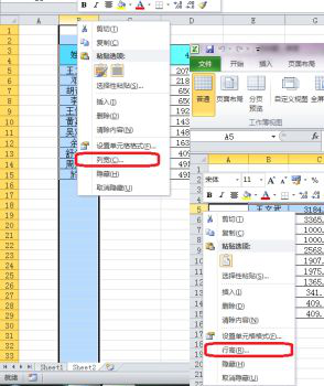
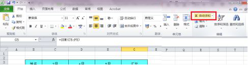
2. Automatic summation of data

Select the cell where the data is located and a blank cell, and then click the summation symbol. Automatic summation.

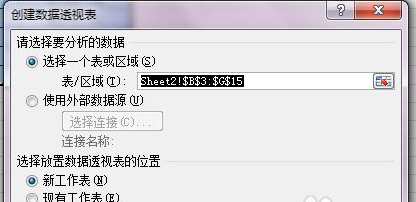
3. Pivot table

Select the entire table and click Insert-Pivot table to insert the Pivot table. Through the Pivot table, you can Implement data aggregation operations.

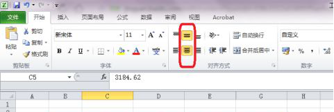
4. Alignment setting

Select the cells that need to be aligned and select the required alignment in the alignment to align the data.

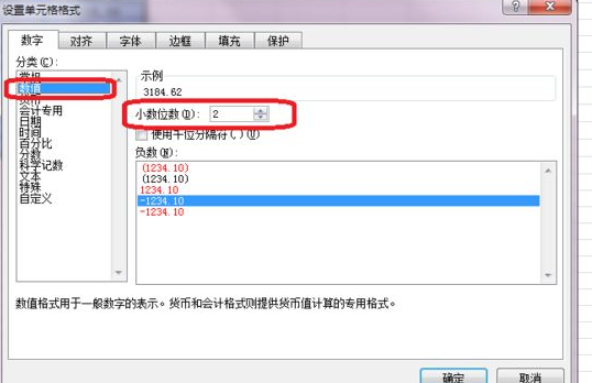
5. Set the number of decimal places to be retained

Select the cells that need to retain decimal places, right-click and select Format Cells, and a dialog box will pop up. Numeric value, set the number of decimal places.

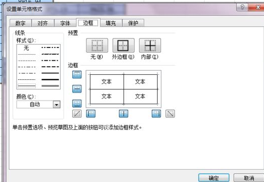
6. Set the table border

Select the table, right-click the mouse and select Format Cells, select the border, and set the table border as needed.

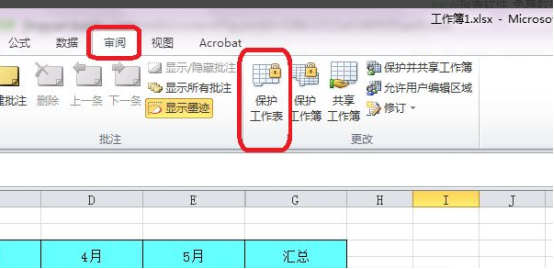
7. Worksheet Encryption

Click "Review"-"Protect Worksheet" directly and enter the password in the pop-up dialog box.

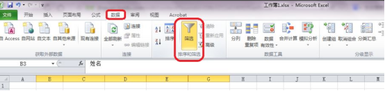
8. Data filtering and sorting

Select the header row of the table, select - "Data" - "Filter", click filter to achieve sorting and sorting Filter function.

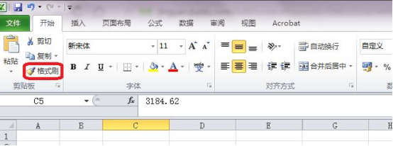
9. Format Painter Quickly Sets Table Format

Select the cells that have been formatted, click the format painter picture, and then click on other cells You can set cell formats by clicking once and double-clicking continuously.

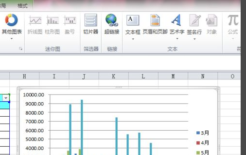
10. Convert data into charts

Select the cells that need to be converted, click "Insert", select a chart style from the chart and click After the insertion is completed, if you need to change the data, you can change the data source by right-clicking "Select Data".

The above is the detailed content of Basic tutorial on using excel. For more information, please follow other related articles on the PHP Chinese website!