A simple tutorial on making a rectangular scatter plot in Excel

A simple tutorial on making scatter plots in Excel Today, PHP editor Xinyi will introduce to you how to use Excel to quickly create a scatter chart. Scatter chart is a very intuitive chart form that shows the relationship between data points. By setting the data source and chart options in Excel, you can easily generate a beautiful scatter chart. Follow the editor's steps and let's learn how to make it!

1. Select the data area - click Insert - Recommended chart - Scatter chart.

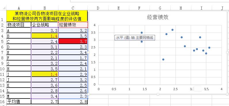
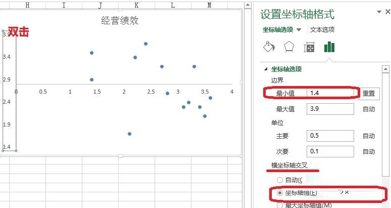
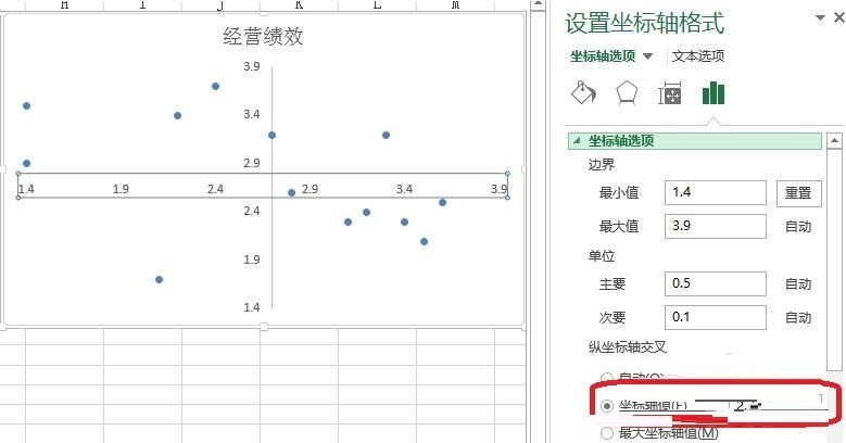
#2. As shown in the figure, double-click the coordinate axis - set the coordinate axis format - the horizontal axis crosses 2.8, and the vertical axis crosses 2.7.

3. Right-click - Add data label.

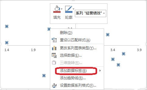
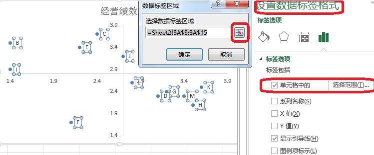
4. Double-click the data label - set the data label format - select the range (A, B...logistics items).

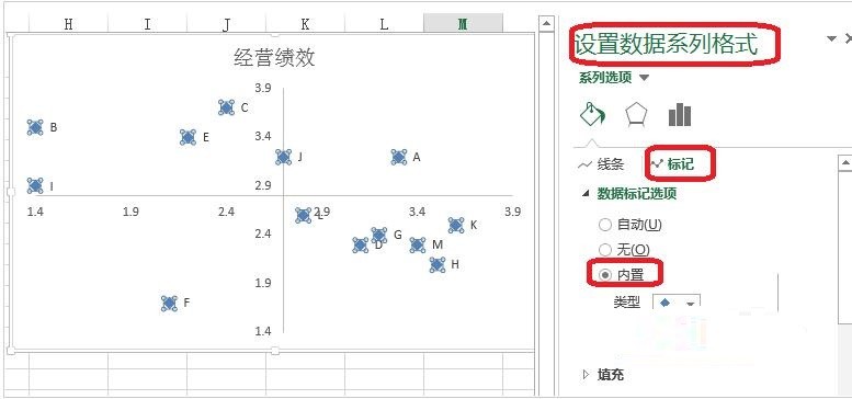
5. As shown in the figure, set the data series format - mark - built-in - size (adjust the size of the data mark).

2. Beautify the chart

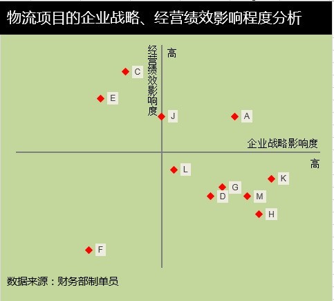
As shown in the figure, beautify the chart and it is easy to see which project has a high impact on business performance and which company has a high strategic impact.

The above is the detailed content of A simple tutorial on making a rectangular scatter plot in Excel. For more information, please follow other related articles on the PHP Chinese website!