
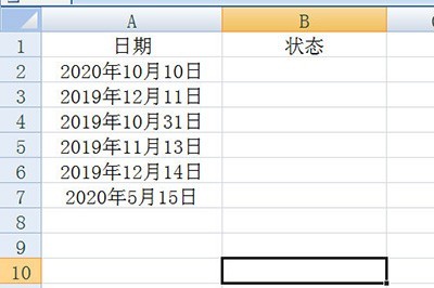
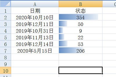
Take the following table as an example. Note that the cell format in the date column is date.
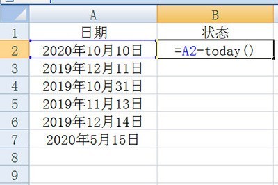
Enter the calculation formula =date column-today() in the status column next to it. That is, the expiration time minus the time of day.
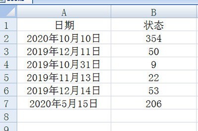
Press Enter to calculate, then drag and drop to all cells below. and change the cell format to regular.
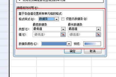
Select this column and click [Start]-[Conditional Formatting]-[New Rule]. In the window, [Format Style] is set to data bar, the shortest data bar in the type is set to the lowest value, and the longest data bar is set to the highest value. Then set the color of the data bar you like.
After clicking OK, an intuitive table of expiry days will be ready.
The above is the detailed content of How to calculate expiration days in Excel. For more information, please follow other related articles on the PHP Chinese website!
 How to turn off win10 upgrade prompt
 The difference between lightweight application servers and cloud servers
 CMD close port command
 The difference between external screen and internal screen broken
 How to jump with parameters in vue.js
 Cell sum
 How to intercept harassing calls
 virtual digital currency


