Review! Deep model fusion (LLM/basic model/federated learning/fine-tuning, etc.)

In September 23, the paper "Deep Model Fusion: A Survey" was published by the National University of Defense Technology, JD.com and Beijing Institute of Technology.

Deep model fusion/merging is an emerging technology that combines the parameters or predictions of multiple deep learning models into a single model. It combines the capabilities of different models to compensate for the biases and errors of individual models for better performance. Deep model fusion on large-scale deep learning models (such as LLM and basic models) faces some challenges, including high computational cost, high-dimensional parameter space, interference between different heterogeneous models, etc. This paper divides existing deep model fusion methods into four categories: (1) "Pattern connection", which connects solutions in the weight space through a loss-reducing path to obtain better model fusion initialization; (2) " Alignment", matching units between neural networks to create better conditions for fusion; (3) "Weight average" is a classic model fusion method that averages the weights of multiple models to obtain a closer optimal solutions and more accurate results; (4) "Ensemble learning" combines the output of different models, which is a basic technology to improve the accuracy and robustness of the final model. In addition, the challenges faced by deep model fusion are analyzed and possible research directions for future model fusion are proposed.

Deep model fusion has attracted increasing interest due to data privacy and practical data saving issues. Although the development of deep model fusion has brought many technological breakthroughs, it has also created a series of challenges, such as high computational load, model heterogeneity, and slow combinatorial optimization alignment. This inspired scientists to study the principles of model fusion in different situations.

Some works only focus on model fusion from a single perspective (such as feature fusion, etc.) [45,195] and specific scenes [213], rather than parameter fusion. Together with recent advances and representative applications, such as federated learning (FL) [160] and fine-tuning [29], this paper divides them into four categories based on internal mechanisms and purposes. The diagram shows a schematic diagram of the entire model fusion process, as well as the classification and connection of various methods.

For models trained independently and not adjacent to each other, "Mode Join" and "Align" bring the solutions closer, resulting in better average raw conditions. For similar models with certain differences in weight spaces, "weight average (WA)" tends to average the models directly to obtain a solution closer to the optimal point in the parameter space region with lower loss function values. Additionally, for predictions from existing models, “ensemble learning” integrates predictions from different forms of the model to achieve better results.

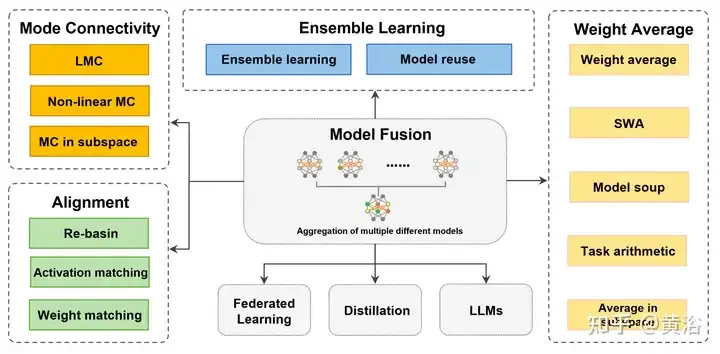
"Model fusion, as a technique to improve the accuracy and robustness of deep models, has promoted improvements in many application areas. 'Federated learning [160]' is a Applications that aggregate model accuracy and robustness of client models on a central server, enabling parties to contribute data to the computation of functions (e.g. various statistics, classifiers [177]) without introducing privacy leaks Risks. 'Fine-tuning' makes small adjustments to a pre-trained model and combines it with model fusion to reduce training costs and adapt to the needs of a specific task or domain. Model fusion also involves 'distillation', that is, combining multiple complex models. Soft target knowledge (teacher), training a small model (student) to adapt to specific needs. 'Model fusion on base/LLM' includes work on large base models or large language models (LLM), such as Transformer (ViT) [ 79], GPT [17], etc. The application of model fusion helps developers adapt to the needs of various tasks and fields, and promotes the development of deep learning." The word count is full.

To determine whether the results of the trained network are stable to SGD noise, The loss barrier (error barrier) is defined as the maximum difference between the two-point loss linear interpolation and the two-point linear connection loss [ 50]. The loss barrier specifies whether the error is constant or increasing along the path optimization graph [56, 61] between W1 and W2. If there is a tunnel between two networks with a barrier approximately equal to 0, it is equivalent to a mode connection [46, 59, 60]. In other words, the local minima obtained by SGD can be connected through a path φ that minimizes the maximum loss.

Solutions obtained by gradient-based optimization can be connected in the weight space through paths (connectors) without barriers, which is called pattern connection[46, 50]. Other models more suitable for model fusion can be obtained along the low-loss path. According to the mathematical form of the path and the space where the connector is located, it is divided into three parts: "Linear Mode Connection (LMC) [66]", "Nonlinear Mode Connection" and "Pattern Connection of Subspace".

Pattern connection can solve the local optimization problem during the training process. The geometric relationships of pattern connection paths [61, 162] can also be used to accelerate the convergence, stability, and accuracy of optimization processes such as stochastic gradient descent (SGD). In summary, pattern connection provides a new perspective for interpreting and understanding the behavior of model fusion [66]. However, computational complexity and parameter tuning difficulties should be addressed, especially when training models on large datasets. The following table is a summary of the standard training procedures for Linear Mode Connection (LMC) and Nonlinear Mode Connection.

The picture shows a schematic diagram of the pattern connection in the two-dimensional loss map and other dimensional subspaces. Left: Linear interpolation of two basin minima results in a high loss barrier [46]. The lower two optimal values ​​follow nearly constant low-loss paths (e.g. Bezier curves, polybox chains, etc.) [66]. π(W2) is the equivalent model of the arrangement symmetry of W2, which is located in the same basin as W1. Re-Basin merges models by providing solutions for individual watersheds [3]. Right: Low-loss paths connect multiple minima in a subspace (e.g., a low-loss manifold consisting of d-dimensional wedges [56], etc.).

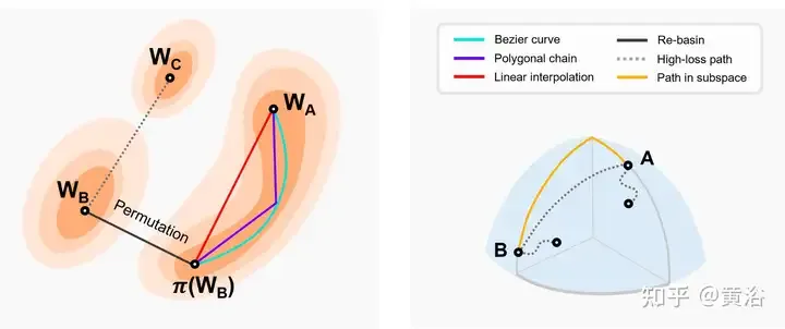
The following table is a method for finding tunnels between different local minima.

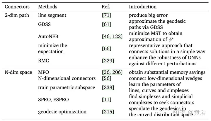
#In short, pattern connection provides a newer and more flexible perspective for deep model fusion. The training of neural networks can easily fall into local optimality, leading to performance degradation. On the basis of model connection, other models with better performance can be found and used as a starting point for further optimization and fusion. The already trained model can be used to move in the parameter space to reach a new target model, which can save time and computational overhead and is suitable for situations where data is limited. However, when connecting different models, additional complexity and flexibility may be introduced, increasing the risk of overfitting. Therefore, the relevant hyperparameters and degree of variation should be carefully controlled. Additionally, pattern concatenation requires fine-tuning or parameter changes, which may increase training time and resource consumption. In summary, model connectivity has many advantages in model fusion, including helping to overcome local optimal problems and providing new perspectives for explaining network behavior. In the future, pattern connection is expected to help understand the internal mechanisms of neural networks and provide guidance for more efficient deep model fusion designs in the future.

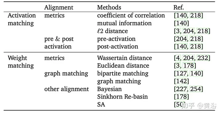
Due to the randomness of channels and components from different networks, the active components of the network interfere with each other [204]. Therefore, misaligned weighted averages may ignore the correspondence between units in different models and corrupt useful information. For example, there is a relationship between two neurons in different models that may be completely different but functionally similar. Alignment is to match units of different models to obtain better initial conditions for deep model fusion. The purpose is to make the differences between multiple models smaller, thereby enhancing the deep model fusion effect. Furthermore, alignment can essentially be viewed as a combinatorial optimization problem. A representative mechanism "Re-basin" that provides solutions for individual basins, merging models with better original conditions. Depending on whether the alignment target is data-driven or not, alignment is divided into two types: "activation matching" and "weight matching", as shown in the table.

Generally speaking, even for shallow neural networks, the number of saddle points and local optima grows exponentially with the number of parameters [10, 66]. It has been found that there is invariance in training, resulting in some points in these local optima having the same representation [22, 81, 140]. Specifically, if the units of the hidden layer are swapped by permutation, the functionality of the network does not change, which is called permutation symmetry[43, 50].

The permutation symmetry brought by these invariants helps to better understand the structure of the loss graph [22, 66]. Invariance can also be viewed as a source of saddle points in the loss graph [14]. [68] study the algebraic structure of symmetries in neural networks and how this structure manifests itself in loss graph geometry. [14] introduced permutation points in high-dimensional platforms where neurons can be swapped without increasing losses or parameter jumps. Perform gradient descent on the loss, adjusting the parameter vectors θm and θn of neurons m and n until the vectors reach the alignment point.

Based on permutation symmetry, solutions in different regions in the weight space can generate equivalent solutions. The equivalent solution is located in the same region as the original solution, with a low-loss barrier (basin), called the "Re-basin" [3]. Compared to pattern connections, re-basin tends to transport points into the basin via alignment rather than low-loss tunneling. Currently, alignment is the representative method of Re-basin [3, 178]. However, how to efficiently search all possibilities of permutation symmetries such that all solutions point to the same basin is a current challenge.

The picture is a schematic diagram of [14] introducing arrangement point exchange neurons. Left: General alignment process, model A is transformed into model Ap with reference to model B, and then the linear combination of Ap and B produces C. Right: Adjust the parameter vectors θm and θn of two neurons in different hidden layers close to the alignment point. At the alignment point [14] θ′m = θ′n, the two neurons calculate the same function, which means that the two neurons Can be exchanged.

Alignment can improve the information sharing between models by adjusting the parameters of the model to make the models more similar, thereby improving the generalization ability of the fusion model. Additionally, alignment helps improve model performance and robustness on complex tasks. However, alignment methods face the problem of slow combinatorial optimization. Alignment requires additional computational overhead to adjust the parameters of the model, which may lead to a more complex and time-consuming training process, especially in large depth models [142, 204].

To sum up, alignment can improve the consistency and overall effect between different models. With the diversification of DL application scenarios, alignment will become one of the key methods to optimize deep model fusion and improve generalization capabilities. In the future, alignment can play a role in transfer learning, domain adaptation [63], knowledge distillation and other fields. For example, alignment can reduce the difference between the source and target domains in transfer learning and improve learning of new domains.

Due to the high redundancy of neural network parameters, there is usually no one-to-one correspondence between the weights of different neural networks. Therefore, weighted averaging (WA) is generally not guaranteed to perform well by default. Ordinary averaging performs poorly for trained networks with large differences in weights [204]. From a statistical perspective, WA allows control of individual model parameters in the model, thereby reducing the variance of the final model and thus having a reliable impact on the regularization properties and output results [77, 166].

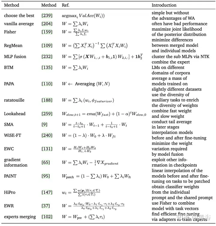
The following table is a representative method of WA:

Subject to Fast Geometry Integration ( Inspired by FGE) [66] and checkpoint averaging [149], [99] utilizes a constant or periodic learning rate to average multiple points of the SGD trajectory, which is regarded as stochastic weight averaging (SWA). SWA improves training on a range of important baselines, providing better temporal scalability. Instead of training a collection of models (like normal fusion), SWA trains a single model to find a smoother solution than SGD. The SWA-related methods are listed in the following table. Furthermore, SWA can be applied to any architecture or data set and demonstrates better performance than Snapshot Integration (SSE) [91] and FGE. At the end of each period, the SWA model is updated by averaging the newly obtained weights with the existing weights.

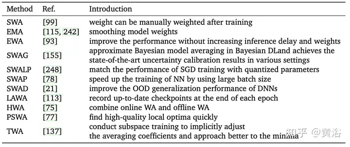
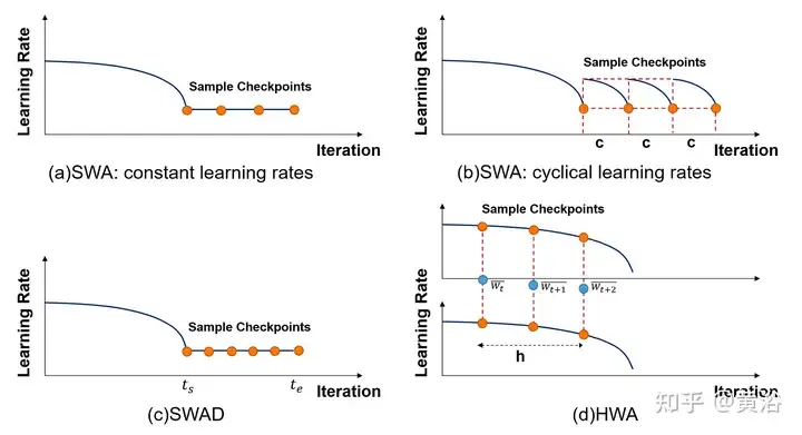
However, SWA can only average points near the local optimal point, and finally obtains a relative minimum value, but cannot accurately approximate the optimal value. In addition, due to certain factors (such as poor early convergence, high learning rate, fast weight change rate, etc.), the final input sample deviation may be large or insufficient, resulting in poor overall results. Extensive work tends to change SWA sampling methods.

As shown in the figure, the sampling and learning rate arrangements of different SWA related methods are compared. (a) SWA: constant learning rate. (b)SWA: Periodic learning rate. (c)SWAD: dense sampling. (d) HWA: Using online and offline WA, sampling at different synchronization periods, the sliding window length is h.

Model soup [239] refers to a method of averaging models fine-tuned with different hyperparameters. It is simple but effective, achieving 90.94% accuracy on ImageNet-1K, surpassing previous work on CoAtNet-7 (90.88%) [38] and ViT-G (90.45%) [255]. The table summarizes the different model soup methods.

In multi-task learning (MTL), the pre-trained model and task vector (i.e. τi = Wft − Wpre, the difference between the pre-trained model and the fine-tuned model) are combined to obtain better performance on all tasks. Based on this observation, Task Arithmetic[94] improves the performance of the model on tasks by fine-tuning task vectors through addition and linear combination, which has become a flexible and efficient method for directly editing pre-trained models, as shown in Figure Display: Using task arithmetic and LoraHub (Low-rank adaptations Hub).

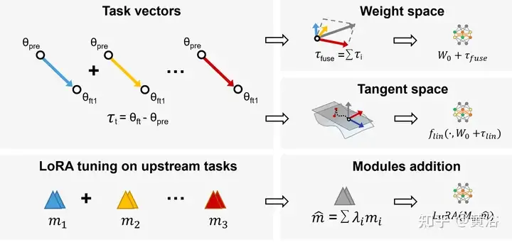
In addition, model fusion in subspace limits the training trajectory to a low-dimensional subspace, which can reduce load and difficulty.

WA obtains the final model by averaging the weights of different depth models without additional computational complexity or training process [109, 159]. In general, if the random models differ significantly in representation capabilities, structure, or training data, the results of the fusion may not achieve the expected performance. Linear interpolation of a model from scratch using the same hyperparameter configuration but with a different data order is even less effective than a stochastic model [59]. Therefore, a large number of proposed methods aim to optimize the WA process in other mathematical ways.

Additionally, when models share part of their optimization trajectory (e.g., checkpoint averaging, tail averaging, SWA [99, 149], etc.) or are fine-tuned on the same pre-trained model (e.g., model soup [239] etc.), the accuracy of the interpolation model performs better [167]. Furthermore, Model Soup [239] averages models with different hyperparameter configurations to obtain the final result. Additionally, choosing appropriate weights in model averaging can also be a challenge, which is often fraught with subjectivity. More complex weight selection mechanisms may require extensive and complex experiments and cross-validation.

WA is a promising technology in deep learning. In the future, it can be used as a model optimization technology to reduce weight fluctuations between different iterations and improve stability and convergence speed. WA can improve the aggregation stage of federated learning (FL) to better protect privacy and reduce future communication costs. In addition, by implementing network compression on the end device, it is expected to reduce the storage space and computational overhead of the model on resource-constrained devices [250]. In short, WA is a promising and cost-effective DL technology that can be applied in areas such as FL to improve performance and reduce storage overhead.

Ensemble learning, or multiple classifier systems, is a technique that integrates multiple single models to generate a final prediction, including voting, averaging [195], etc. It improves the overall performance and reduces the variance of the model, solving problems such as overfitting, instability, and limited data volume.

Based on existing pre-trained source models, Model reuse[266] provides the models needed to be applied to new tasks without the need to retrain a new model from scratch. It saves time and computing resources and provides better performance under limited resource conditions [249]. In addition, since the focus of transfer learning is to solve the prediction task on the target domain, model reuse can be regarded as a type of transfer learning. However, transfer learning requires labeled data from the source domain and the target domain, while in model reuse, only unlabeled data can be collected, but data from the source domain cannot be used [153].

Unlike multi-classifier ensemble learning, most current methods reuse existing features, labels, or modalities to obtain final predictions [176, 266] without storing large amounts of training data [245]. Another key challenge in model reuse is identifying useful models from a set of pretrained models for a given learning task.

Using a single model for model reuse will produce too much homogeneous information (e.g., a model trained in one domain may not fit the data of another domain), and it is difficult to find a single predictor that fully fits the target domain. Train the model. In general, using a set of similar models to produce better performance than a single model is denoted as Multiple Model Reuse (MMR)[153].

The following table compares the characteristics of different reuse methods. In short, model reuse can significantly reduce the amount of data required to use pre-trained models and solve the problem of consuming a large amount of bandwidth when transmitting data between different ends. question. Multi-model reuse also has a wide range of applications, such as speech recognition, secure and private interaction systems, digital retina [64], etc.

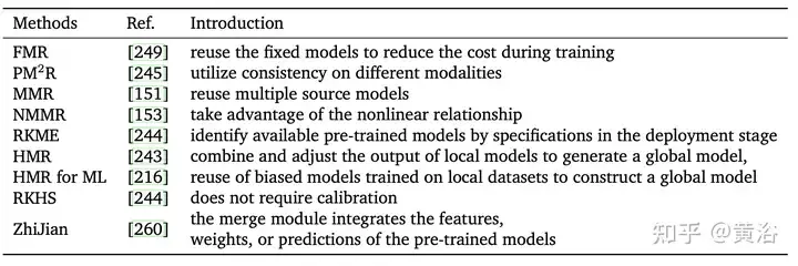
Compared with related model fusion algorithms such as federated learning [88,89,160] which have certain requirements on model parameters and scale, ensemble learning method utilizes Prediction to combine multiple heterogeneous weak classifiers has no such limitation. In addition, networks with different architectures in the integration method will have more obvious comparison effects than WA. However, ensemble approaches require maintaining and running multiple trained models and running them together at test time. Considering the size and complexity of deep learning models, this approach is not suitable for applications with limited computing resources and costs [204].

Due to the diversity of the ensemble learning framework, model diversity can be achieved and generalization capabilities can be enhanced. In the future, this will be important for handling data changes and adversarial attacks. Ensemble learning in deep learning is expected to provide confidence estimates and uncertainty measures for model predictions, which are crucial for the safety and reliability of decision support systems, autonomous driving [74], medical diagnosis, etc.

In recent years, a large amount of new research has appeared in the field of deep model fusion, which has also promoted the development of related application fields.

Federated Learning

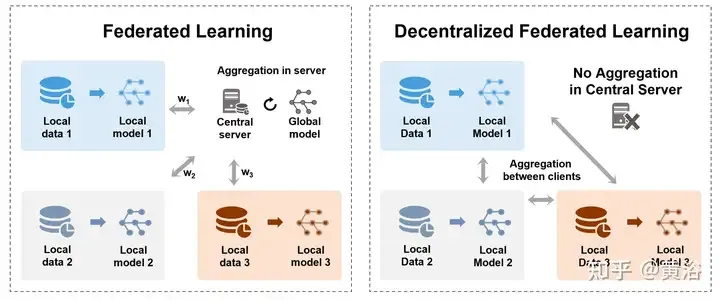
To address the security and centralization challenges of data storage, federated learning (FL) [160, 170] allows many participating models to collaboratively train shared Global model while preserving data privacy without centralizing datasets on a central server. It can also be viewed as a multi-party learning problem [177]. In particular, Aggregation is an important process of FL, which contains model or parameter updates trained by various parties (such as devices, organizations, or individuals). The figure demonstrates two different aggregation methods in centralized and decentralized FL. , Left: Centralized federated learning between a central server and client terminals, transferring models or gradients and finally aggregating on the server. Right: Decentralized federated learning transfers and aggregates models between client terminals without the need for a central server.

The following table is the different aggregation methods of federated learning:

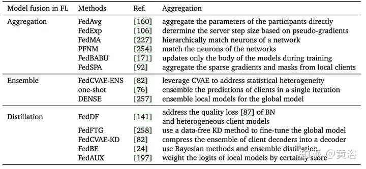
In short, the aggregation step in FL Essentially it is a model fusion technology. Choosing a reasonable model fusion method can reduce the impact of specific participant or individual data on the final model, thereby improving the model's generalization ability and adaptability in the global scope. Good aggregation methods are expected to help address a range of challenges in federated learning in the future. High-quality and scalable aggregation methods are expected to face a series of challenges of FL, such as client heterogeneity, non-IID heterogeneous data, limited computing resources [141], etc. FL is expected to show its potential in more fields, such as natural language processing, recommendation systems [146], medical image analysis [144], etc.

Fine-tuning

Fine-tuning is a basic pattern (such as a pre-trained model) and is an effective way to adjust the model to perform downstream tasks [23, 41], which can be used Less labeled data results in better generalization and more accurate output. Pretrained models are trained with a relatively task-specific set of data, which is always a better starting point for training criteria than random initialization. despite this. On average, existing fine-tuned models [28, 29] are even better base models than ordinary pre-trained models for fine-tuning downstream tasks.

In addition, there are a lot of recent works that combine WA with fine-tuning, as shown in the figure, such as model soup [239], DiWA [190], etc. Fine-tuning improves the accuracy of the target distribution, but often results in reduced robustness to distribution changes. Strategies for averaging fine-tuned models may be simple, but they do not fully exploit the connections between each fine-tuned model. Therefore, training on intermediate tasks before training on the target task can explore the capabilities of the base model [180, 185, 224]. Inspired by the mutual training strategy [185], [188] fine-tune the model for auxiliary tasks to exploit different auxiliary tasks and improve out-of-distribution (OOD) generalization capabilities.

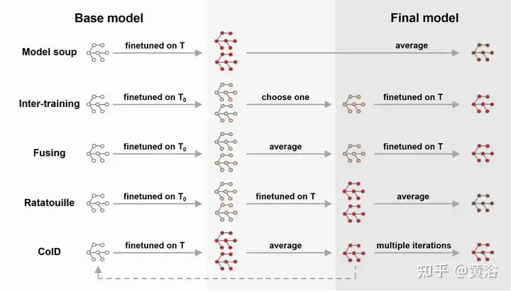
Fine-tuning the average of the model reduces the training time required to achieve the goal [28] and produces a more accurate and better generalized model. Essentially, different fine-tuning methods (for example, frozen layer fine-tuning, top-level fine-tuning, etc.) will also have a certain impact on the final accuracy and distribution shift [240]. However, the combination of WA and fine-tuning is expensive and has certain limitations on specific applications. Furthermore, it may face the problem of saved checkpoint explosion or catastrophic forgetting [121], especially when applied to transfer learning.

Knowledge Distillation

Knowledge distillation (KD) [83] is an important method for integrating multiple models, involving the following two types of models. Teacher model refers to a large and powerful model trained on large-scale data, with high predictive and expressive capabilities. Student model is a relatively small model with fewer parameters and computational resources [18, 199]. Using the teacher's knowledge (such as output probability distribution, hidden layer representation, etc.) to guide training, students can achieve predictive capabilities close to large models with fewer resources and faster speed [2, 119, 124, 221]. Considering that multiple teachers or students are expected to perform better than a single model [6], KD is divided into two categories based on the aggregation objective, as shown in the figure.

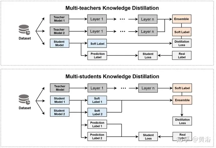
The first type of method is to merge multiple teacher models and directly extract the student model, as shown in the table. Currently, recent work mainly integrates the output of teachers (e.g., logits [6, 49, 252] or feature base knowledge [143, 241], etc.).

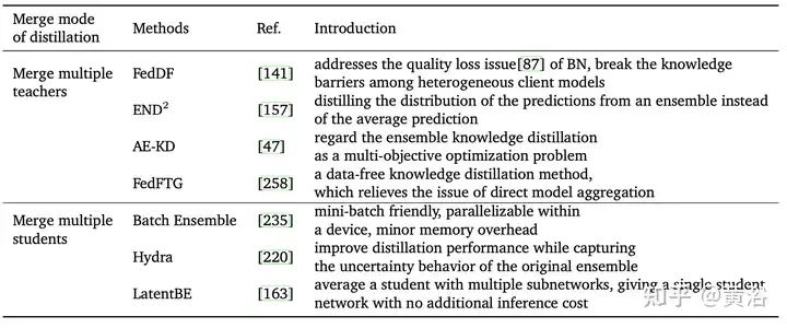
Another approach is to use a teacher model to extract multiple students and then merge these student models. However, merging multiple students also has some problems, such as high computational resource requirements, poor interpretability, and over-reliance on the original model.

Model fusion of basic models/LLMs

Basic models show strong performance and emergent capabilities when processing complex tasks. The characteristic of large-scale basic models is their huge Scale, containing billions of parameters, helps learn complex patterns in data. Especially, with the recent emergence of new LLMs [200, 264], such as GPT-3 [17, 172], T5 [187], BERT [41], Megatron-LM, WA applications [154, 212, 256 ] ] LLM attracted more attention.

In addition, recent works [120, 256] tend to design better frameworks and modules to adapt to apply LLM. Due to high performance and low computational resources, fine-tuning large base models can improve robustness to distribution changes [240].

The above is the detailed content of Review! Deep model fusion (LLM/basic model/federated learning/fine-tuning, etc.). For more information, please follow other related articles on the PHP Chinese website!