Identify overfitting and underfitting through learning curves
This article will introduce how to effectively identify overfitting and underfitting in machine learning models through learning curves.
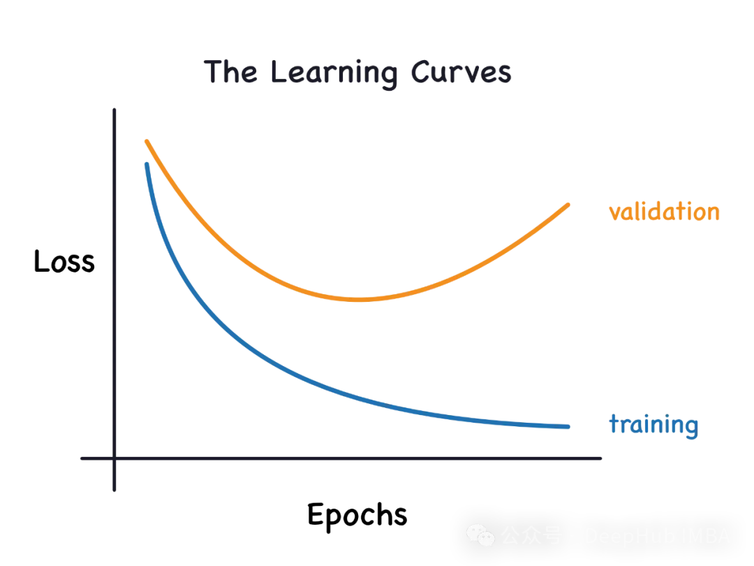
Underfitting and overfitting
1. Overfitting
If a model is overtrained on data to the point that it learns noise from it, the model is said to be overfitted. An overfitted model learns every example so perfectly that it will misclassify an unseen/new example. For an overfitted model, we will get a perfect/near-perfect training set score and a terrible validation set/test score.
Slightly modified: "The reason for overfitting: Use a complex model to solve a simple problem and extract noise from the data. Because a small data set may not be used as a training set Represents the correct representation of all data. "
2. Underfitting
If a model cannot correctly learn the patterns in the data, we Let's just say it's underfitting. Underfitting models do not fully learn every example in the data set. In this case, we see that the errors on both the training and validation sets are low. This may be because the model is too simple and does not have enough parameters to fit the data. We can try to increase the complexity of the model, increase the number of layers or neurons, to solve the under-fitting problem. However, it should be noted that increasing model complexity also increases the risk of overfitting.
Reasons why it is not suitable: Using a simple model to solve a complex problem, the model cannot learn all the patterns in the data, or the model incorrectly learns the patterns of the underlying data. In data analysis and machine learning, model selection is very important. Choosing the right model for your problem can improve the accuracy and reliability of your predictions. For complex problems, more complex models may be needed to capture all patterns in the data. In addition, you also need to consider the
learning curve
The learning curve draws the training sum of the training sample itself by incrementally adding new training samples. Verification loss. Can help us determine if we need to add additional training examples to improve the validation score (score on unseen data). If the model is overfitted, then adding additional training examples may improve the model's performance on unseen data. Likewise, if a model is underfit, then adding training examples may not be useful. The 'learning_curve' method can be imported from Scikit-Learn's 'model_selection' module.
from sklearn.model_selection import learning_curve
We will demonstrate using logistic regression and Iris data. Create a function called "learn_curve" that will fit a logistic regression model and return cross-validation scores, training scores, and learning curve data.
#The function below builds the model and returns cross validation scores, train score and learning curve data def learn_curve(X,y,c): ''' param X: Matrix of input featuresparam y: Vector of Target/Labelc: Inverse Regularization variable to control overfitting (high value causes overfitting, low value causes underfitting)''' '''We aren't splitting the data into train and test because we will use StratifiedKFoldCV.KFold CV is a preferred method compared to hold out CV, since the model is tested on all the examples.Hold out CV is preferred when the model takes too long to train and we have a huge test set that truly represents the universe''' le = LabelEncoder() # Label encoding the target sc = StandardScaler() # Scaling the input features y = le.fit_transform(y)#Label Encoding the target log_reg = LogisticRegression(max_iter=200,random_state=11,C=c) # LogisticRegression model # Pipeline with scaling and classification as steps, must use a pipelne since we are using KFoldCV lr = Pipeline(steps=(['scaler',sc],['classifier',log_reg])) cv = StratifiedKFold(n_splits=5,random_state=11,shuffle=True) # Creating a StratifiedKFold object with 5 folds cv_scores = cross_val_score(lr,X,y,scoring="accuracy",cv=cv) # Storing the CV scores (accuracy) of each fold lr.fit(X,y) # Fitting the model train_score = lr.score(X,y) # Scoring the model on train set #Building the learning curve train_size,train_scores,test_scores =learning_curve(estimator=lr,X=X,y=y,cv=cv,scoring="accuracy",random_state=11) train_scores = 1-np.mean(train_scores,axis=1)#converting the accuracy score to misclassification rate test_scores = 1-np.mean(test_scores,axis=1)#converting the accuracy score to misclassification rate lc =pd.DataFrame({"Training_size":train_size,"Training_loss":train_scores,"Validation_loss":test_scores}).melt(id_vars="Training_size") return {"cv_scores":cv_scores,"train_score":train_score,"learning_curve":lc}The above code is very simple, it is our daily training process. Now we start to introduce the use of learning curve
1. Learning curve of the fitted model
We will use the 'learn_curve' function to obtain a good fitted model by setting the anti-regularization variable/parameter 'c' to 1 (i.e. we don't perform any regularization).
lc = learn_curve(X,y,1) print(f'Cross Validation Accuracies:\n{"-"*25}\n{list(lc["cv_scores"])}\n\n\ Mean Cross Validation Accuracy:\n{"-"*25}\n{np.mean(lc["cv_scores"])}\n\n\ Standard Deviation of Deep HUB Cross Validation Accuracy:\n{"-"*25}\n{np.std(lc["cv_scores"])}\n\n\ Training Accuracy:\n{"-"*15}\n{lc["train_score"]}\n\n') sns.lineplot(data=lc["learning_curve"],x="Training_size",y="value",hue="variable") plt.title("Learning Curve of Good Fit Model") plt.ylabel("Misclassification Rate/Loss");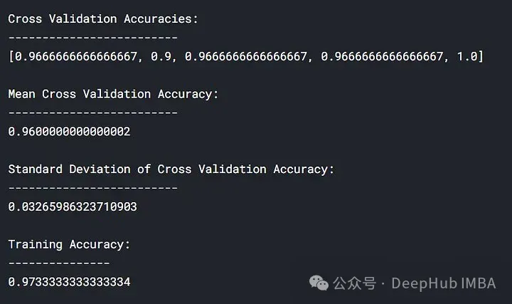
#In the above results, the cross-validation accuracy is close to the training accuracy.
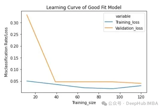
Training loss (blue): The learning curve of a good fitted model will gradually decrease and decrease as the number of training examples increases. It gradually becomes flat, indicating that adding more training examples does not improve the model's performance on the training data.
Validation loss (yellow): The learning curve of a well-fitted model has a high validation loss at the beginning, which gradually decreases and gradually decreases as the number of training examples increases. tends to be flat, indicating that the more samples, the more patterns can be learned. These patterns will be helpful for "unseen" data
Finally, you can also see that in After adding a reasonable number of training examples, the training loss and validation loss approach each other.
2. Learning Curve of Overfitting Model
We will use the 'learn_curve' function by deregularizing the variable/parameter 'c 'Set to 10000 to get an overfitted model (high values of 'c' result in overfitting).
lc = learn_curve(X,y,10000) print(f'Cross Validation Accuracies:\n{"-"*25}\n{list(lc["cv_scores"])}\n\n\ Mean Cross Validation Deep HUB Accuracy:\n{"-"*25}\n{np.mean(lc["cv_scores"])}\n\n\ Standard Deviation of Cross Validation Accuracy:\n{"-"*25}\n{np.std(lc["cv_scores"])} (High Variance)\n\n\ Training Accuracy:\n{"-"*15}\n{lc["train_score"]}\n\n') sns.lineplot(data=lc["learning_curve"],x="Training_size",y="value",hue="variable") plt.title("Learning Curve of an Overfit Model") plt.ylabel("Misclassification Rate/Loss");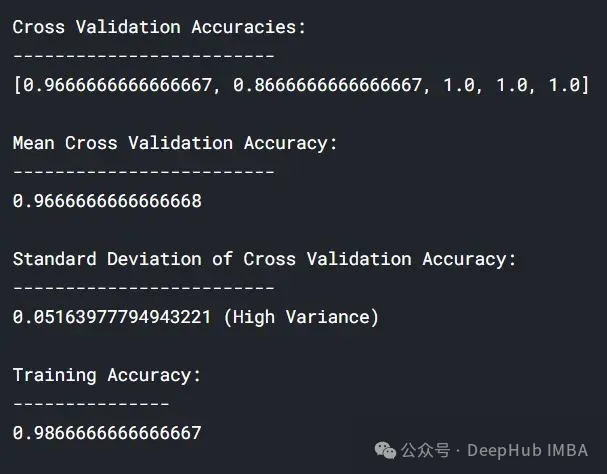
与拟合模型相比,交叉验证精度的标准差较高。
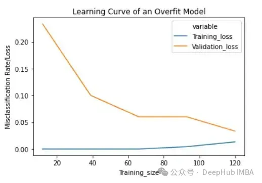
过拟合模型的学习曲线一开始的训练损失很低,随着训练样例的增加,学习曲线逐渐增加,但不会变平。过拟合模型的学习曲线在开始时具有较高的验证损失,随着训练样例的增加逐渐减小并且不趋于平坦,说明增加更多的训练样例可以提高模型在未知数据上的性能。同时还可以看到,训练损失和验证损失彼此相差很远,在增加额外的训练数据时,它们可能会彼此接近。
3、欠拟合模型的学习曲线
将反正则化变量/参数' c '设置为1/10000来获得欠拟合模型(' c '的低值导致欠拟合)。
lc = learn_curve(X,y,1/10000) print(f'Cross Validation Accuracies:\n{"-"*25}\n{list(lc["cv_scores"])}\n\n\ Mean Cross Validation Accuracy:\n{"-"*25}\n{np.mean(lc["cv_scores"])}\n\n\ Standard Deviation of Cross Validation Accuracy:\n{"-"*25}\n{np.std(lc["cv_scores"])} (Low variance)\n\n\ Training Deep HUB Accuracy:\n{"-"*15}\n{lc["train_score"]}\n\n') sns.lineplot(data=lc["learning_curve"],x="Training_size",y="value",hue="variable") plt.title("Learning Curve of an Underfit Model") plt.ylabel("Misclassification Rate/Loss");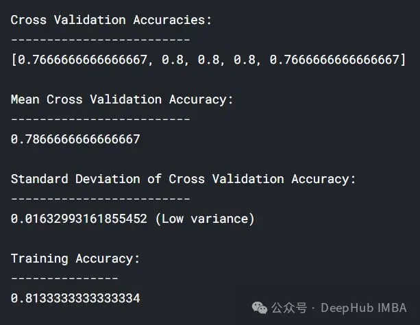
与过拟合和良好拟合模型相比,交叉验证精度的标准差较低。
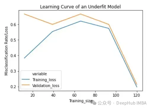
欠拟合模型的学习曲线在开始时具有较低的训练损失,随着训练样例的增加逐渐增加,并在最后突然下降到任意最小点(最小并不意味着零损失)。这种最后的突然下跌可能并不总是会发生。这表明增加更多的训练样例并不能提高模型在未知数据上的性能。
总结
在机器学习和统计建模中,过拟合(Overfitting)和欠拟合(Underfitting)是两种常见的问题,它们描述了模型与训练数据的拟合程度如何影响模型在新数据上的表现。
分析生成的学习曲线时,可以关注以下几个方面:
- 欠拟合:如果学习曲线显示训练集和验证集的性能都比较低,或者两者都随着训练样本数量的增加而缓慢提升,这通常表明模型欠拟合。这种情况下,模型可能太简单,无法捕捉数据中的基本模式。
- 过拟合:如果训练集的性能随着样本数量的增加而提高,而验证集的性能在一定点后开始下降或停滞不前,这通常表示模型过拟合。在这种情况下,模型可能太复杂,过度适应了训练数据中的噪声而非潜在的数据模式。
根据学习曲线的分析,你可以采取以下策略进行调整:
- 对于欠拟合:
- 增加模型复杂度,例如使用更多的特征、更深的网络或更多的参数。
- 改善特征工程,尝试不同的特征组合或转换。
- 增加迭代次数或调整学习率。
- 对于过拟合:
使用正则化技术(如L1、L2正则化)。
减少模型的复杂性,比如减少参数数量、层数或特征数量。
增加更多的训练数据。
应用数据增强技术。
使用早停(early stopping)等技术来避免过度训练。
通过这样的分析和调整,学习曲线能够帮助你更有效地优化模型,并提高其在未知数据上的泛化能力。
The above is the detailed content of Identify overfitting and underfitting through learning curves. For more information, please follow other related articles on the PHP Chinese website!

Hot AI Tools

Undresser.AI Undress
AI-powered app for creating realistic nude photos

AI Clothes Remover
Online AI tool for removing clothes from photos.

Undress AI Tool
Undress images for free

Clothoff.io
AI clothes remover

AI Hentai Generator
Generate AI Hentai for free.

Hot Article

Hot Tools

Notepad++7.3.1
Easy-to-use and free code editor

SublimeText3 Chinese version
Chinese version, very easy to use

Zend Studio 13.0.1
Powerful PHP integrated development environment

Dreamweaver CS6
Visual web development tools

SublimeText3 Mac version
God-level code editing software (SublimeText3)

Hot Topics
 1377
1377
 52
52
 Bytedance Cutting launches SVIP super membership: 499 yuan for continuous annual subscription, providing a variety of AI functions
Jun 28, 2024 am 03:51 AM
This site reported on June 27 that Jianying is a video editing software developed by FaceMeng Technology, a subsidiary of ByteDance. It relies on the Douyin platform and basically produces short video content for users of the platform. It is compatible with iOS, Android, and Windows. , MacOS and other operating systems. Jianying officially announced the upgrade of its membership system and launched a new SVIP, which includes a variety of AI black technologies, such as intelligent translation, intelligent highlighting, intelligent packaging, digital human synthesis, etc. In terms of price, the monthly fee for clipping SVIP is 79 yuan, the annual fee is 599 yuan (note on this site: equivalent to 49.9 yuan per month), the continuous monthly subscription is 59 yuan per month, and the continuous annual subscription is 499 yuan per year (equivalent to 41.6 yuan per month) . In addition, the cut official also stated that in order to improve the user experience, those who have subscribed to the original VIP
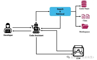 Context-augmented AI coding assistant using Rag and Sem-Rag
Jun 10, 2024 am 11:08 AM
Improve developer productivity, efficiency, and accuracy by incorporating retrieval-enhanced generation and semantic memory into AI coding assistants. Translated from EnhancingAICodingAssistantswithContextUsingRAGandSEM-RAG, author JanakiramMSV. While basic AI programming assistants are naturally helpful, they often fail to provide the most relevant and correct code suggestions because they rely on a general understanding of the software language and the most common patterns of writing software. The code generated by these coding assistants is suitable for solving the problems they are responsible for solving, but often does not conform to the coding standards, conventions and styles of the individual teams. This often results in suggestions that need to be modified or refined in order for the code to be accepted into the application
 Can fine-tuning really allow LLM to learn new things: introducing new knowledge may make the model produce more hallucinations
Jun 11, 2024 pm 03:57 PM
Large Language Models (LLMs) are trained on huge text databases, where they acquire large amounts of real-world knowledge. This knowledge is embedded into their parameters and can then be used when needed. The knowledge of these models is "reified" at the end of training. At the end of pre-training, the model actually stops learning. Align or fine-tune the model to learn how to leverage this knowledge and respond more naturally to user questions. But sometimes model knowledge is not enough, and although the model can access external content through RAG, it is considered beneficial to adapt the model to new domains through fine-tuning. This fine-tuning is performed using input from human annotators or other LLM creations, where the model encounters additional real-world knowledge and integrates it
 Seven Cool GenAI & LLM Technical Interview Questions
Jun 07, 2024 am 10:06 AM
To learn more about AIGC, please visit: 51CTOAI.x Community https://www.51cto.com/aigc/Translator|Jingyan Reviewer|Chonglou is different from the traditional question bank that can be seen everywhere on the Internet. These questions It requires thinking outside the box. Large Language Models (LLMs) are increasingly important in the fields of data science, generative artificial intelligence (GenAI), and artificial intelligence. These complex algorithms enhance human skills and drive efficiency and innovation in many industries, becoming the key for companies to remain competitive. LLM has a wide range of applications. It can be used in fields such as natural language processing, text generation, speech recognition and recommendation systems. By learning from large amounts of data, LLM is able to generate text
 To provide a new scientific and complex question answering benchmark and evaluation system for large models, UNSW, Argonne, University of Chicago and other institutions jointly launched the SciQAG framework
Jul 25, 2024 am 06:42 AM
Editor |ScienceAI Question Answering (QA) data set plays a vital role in promoting natural language processing (NLP) research. High-quality QA data sets can not only be used to fine-tune models, but also effectively evaluate the capabilities of large language models (LLM), especially the ability to understand and reason about scientific knowledge. Although there are currently many scientific QA data sets covering medicine, chemistry, biology and other fields, these data sets still have some shortcomings. First, the data form is relatively simple, most of which are multiple-choice questions. They are easy to evaluate, but limit the model's answer selection range and cannot fully test the model's ability to answer scientific questions. In contrast, open-ended Q&A
 Five schools of machine learning you don't know about
Jun 05, 2024 pm 08:51 PM
Machine learning is an important branch of artificial intelligence that gives computers the ability to learn from data and improve their capabilities without being explicitly programmed. Machine learning has a wide range of applications in various fields, from image recognition and natural language processing to recommendation systems and fraud detection, and it is changing the way we live. There are many different methods and theories in the field of machine learning, among which the five most influential methods are called the "Five Schools of Machine Learning". The five major schools are the symbolic school, the connectionist school, the evolutionary school, the Bayesian school and the analogy school. 1. Symbolism, also known as symbolism, emphasizes the use of symbols for logical reasoning and expression of knowledge. This school of thought believes that learning is a process of reverse deduction, through existing
 SOTA performance, Xiamen multi-modal protein-ligand affinity prediction AI method, combines molecular surface information for the first time
Jul 17, 2024 pm 06:37 PM
Editor | KX In the field of drug research and development, accurately and effectively predicting the binding affinity of proteins and ligands is crucial for drug screening and optimization. However, current studies do not take into account the important role of molecular surface information in protein-ligand interactions. Based on this, researchers from Xiamen University proposed a novel multi-modal feature extraction (MFE) framework, which for the first time combines information on protein surface, 3D structure and sequence, and uses a cross-attention mechanism to compare different modalities. feature alignment. Experimental results demonstrate that this method achieves state-of-the-art performance in predicting protein-ligand binding affinities. Furthermore, ablation studies demonstrate the effectiveness and necessity of protein surface information and multimodal feature alignment within this framework. Related research begins with "S
 Laying out markets such as AI, GlobalFoundries acquires Tagore Technology's gallium nitride technology and related teams
Jul 15, 2024 pm 12:21 PM
According to news from this website on July 5, GlobalFoundries issued a press release on July 1 this year, announcing the acquisition of Tagore Technology’s power gallium nitride (GaN) technology and intellectual property portfolio, hoping to expand its market share in automobiles and the Internet of Things. and artificial intelligence data center application areas to explore higher efficiency and better performance. As technologies such as generative AI continue to develop in the digital world, gallium nitride (GaN) has become a key solution for sustainable and efficient power management, especially in data centers. This website quoted the official announcement that during this acquisition, Tagore Technology’s engineering team will join GLOBALFOUNDRIES to further develop gallium nitride technology. G


