Comment Python Numpy fonctionne sur les tableaux et les matrices

Cette fois, je vais vous montrer comment Python Numpy exploite les tableaux et les matrices. Quelles sont les précautions à prendre pour faire fonctionner les tableaux et les matrices dans Python Numpy. Voici des cas pratiques, jetons un coup d'oeil.

L'objet principal de NumPy est un tableau multidimensionnel d'éléments homogènes. Il s'agit d'un tableau d'éléments dont les éléments sont tous d'un même type, indexés par un tuple d'entiers positifs (généralement les éléments sont des nombres).

Dans NumPy, les dimensions sont appelées axes et le nombre d'axes est appelé rang, mais ce n'est pas la même chose que le rang en algèbre linéaire. Lorsque nous utilisons Python pour trouver le rang en algèbre linéaire, nous utilisons le. linalg.matrix_rank dans le package numpy pour calculer le rang de la matrice, l'exemple est le suivant).

Le résultat est :

La définition du rang en algèbre linéaire : Supposons qu'il y ait un dans matrice A La sous-formule D d'ordre r qui n'est pas égale à 0, et toutes les sous-formules d'ordre r+1 (si elles existent) sont égales à 0, alors D est appelée la sous-formule non nulle d'ordre le plus élevé de la matrice A, et le nombre r est appelé le rang de la matrice A, notons-le R(A).

La différence entre les tableaux et les matrices dans numpy :

La matrice est une branche du tableau. La matrice et le tableau sont courants dans de nombreux cas. .Vous Peu importe celui que vous utilisez. Mais à l'heure actuelle, la recommandation officielle est que si les deux peuvent être utilisés de manière interchangeable, alors choisissez un tableau, car le tableau est plus flexible et plus rapide, et de nombreuses personnes traduisent également des tableaux bidimensionnels en matrices.

Mais l'avantage de la matrice réside dans l'opération relativement simple des symboles. Par exemple, lors de la multiplication de deux matrices, le symbole * est utilisé. Cependant, la multiplication par tableau ne peut pas être utilisée de cette manière. .dot()

L'avantage du tableau est qu'il représente non seulement deux dimensions, mais aussi 3, 4, 5... dimensions, et dans la plupart des programmes Python, le tableau est également plus couramment utilisé.

Nous discutons maintenant des tableaux multidimensionnels de numpy

Par exemple, les coordonnées [1, 2, 3] d'un point dans l'espace 3D sont un Rank est un tableau de 1 car il n'a qu'un seul axe. Cette longueur d'axe est de 3. Comme autre exemple, dans l'exemple suivant, le tableau a le rang 2 (il a deux dimensions). La première dimension a une longueur de 2 et la deuxième dimension a une longueur de 3.

[[ 1., 0., 0.],
 [ 0., 1., 2.]]

. La classe tableau de NumPy s'appelle ndarray. Souvent appelé tableau. Notez que numpy.array n'est pas la même chose que la classe de bibliothèque Python standard array.array, qui ne gère que les tableaux unidimensionnels et fournit une petite quantité de fonctionnalités. Les attributs d'objet ndarray les plus importants sont :

ndarray.ndim

Le nombre d'axes du tableau Dans le monde python, le nombre d'axes est appelé rang

<.>

ndarray.shape

La dimension du tableau. Il s'agit d'un tuple d'entiers indiquant la taille du tableau dans chaque dimension. Par exemple, pour une matrice avec n lignes et m colonnes, son attribut shape sera (2,3). La longueur de ce tuple est évidemment le rang, c'est-à-dire l'attribut dimension ou ndim

ndarray.size

Le nombre total d'éléments du tableau est égal au produit des éléments du tuple dans l'attribut shape.

ndarray.dtype

Un objet utilisé pour décrire le type d'éléments dans le tableau Les types Python standard peuvent être utilisés en créant ou en spécifiant un dtype. De plus, NumPy fournit ses propres types de données.

ndarray.itemsize

La taille en octets de chaque élément du tableau. Par exemple, la valeur de l'attribut itemsiz d'un tableau avec un type d'élément float64 est 8 (=64/8), et par exemple, la valeur de l'attribut item d'un tableau avec un type d'élément complex32 est 4 (=32/8). .

ndarray.data

Un tampon contenant les éléments réels du tableau, nous n'avons généralement pas besoin d'utiliser cette propriété puisque nous utilisons toujours les éléments du tableau par index .

Un exemple 1

>>> from numpy import *
>>> a = arange(15).reshape(3, 5)
>>> a
array([[ 0, 1, 2, 3, 4],
 [ 5, 6, 7, 8, 9],
 [10, 11, 12, 13, 14]])
>>> a.shape
(3, 5)
>>> a.ndim
2
>>> a.dtype.name
'int32'
>>> a.itemsize
4
>>> a.size
15
>>> type(a)
numpy.ndarray
>>> b = array([6, 7, 8])
>>> b
array([6, 7, 8])
>>> type(b)
numpy.ndarray

Création d'un tableau Il existe plusieurs manières de créer des tableaux.

Par exemple, vous pouvez utiliser la fonction array pour créer des tableaux à partir de listes et de tuples Python classiques. Le type du tableau créé est dérivé des types d'éléments de la séquence d'origine.

Une erreur courante consiste à appeler un tableau avec plusieurs arguments numériques au lieu de fournir une liste de valeurs numériques sous la forme d'un seul argument.

>>> from numpy import *
>>> a = array( [2,3,4] )
>>> a
array([2, 3, 4])
>>> a.dtype
dtype('int32')
>>> b = array([1.2, 3.5, 5.1])
>>> b.dtype
dtype('float64')

Array convertit une séquence contenant une séquence en un tableau bidimensionnel, une séquence contenant une séquence contenant une séquence en un tableau tridimensionnel, etc.

>>> a = array(1,2,3,4) # WRONG
>>> a = array([1,2,3,4]) # RIGHT

Le type de tableau peut être explicitement spécifié lors de la création

>>> b = array( [ (1.5,2,3), (4,5,6) ] )
>>> b
array([[ 1.5, 2. , 3. ],
 [ 4. , 5. , 6. ]])

>>> c = array( [ [1,2], [3,4] ], dtype=complex )
>>> c
array([[ 1.+0.j, 2.+0.j],
 [ 3.+0.j, 4.+0.j]])

通常，数组的元素开始都是未知的，但是它的大小已知。因此，NumPy提供了一些使用占位符创建数组的函数。这最小化了扩展数组的需要和高昂的运算代价。

函数function创建一个全是0的数组，函数ones创建一个全1的数组，函数empty创建一个内容随机并且依赖与内存状态的数组。默认创建的数组类型(dtype)都是float64。

>>> zeros( (3,4) )
array([[0., 0., 0., 0.],
 [0., 0., 0., 0.],
 [0., 0., 0., 0.]])
>>> ones( (2,3,4), dtype=int16 )  # dtype can also be specified
array([[[ 1, 1, 1, 1],
 [ 1, 1, 1, 1],
 [ 1, 1, 1, 1]],
 [[ 1, 1, 1, 1],
 [ 1, 1, 1, 1],
 [ 1, 1, 1, 1]]], dtype=int16)
>>> empty( (2,3) )
array([[ 3.73603959e-262, 6.02658058e-154, 6.55490914e-260],
 [ 5.30498948e-313, 3.14673309e-307, 1.00000000e+000]])

为了创建一个数列，NumPy提供一个类似arange的函数返回数组而不是列表:

>>> arange( 10, 30, 5 )
array([10, 15, 20, 25])
>>> arange( 0, 2, 0.3 )   # it accepts float arguments
array([ 0. , 0.3, 0.6, 0.9, 1.2, 1.5, 1.8])

当arange使用浮点数参数时，由于有限的浮点数精度，通常无法预测获得的元素个数。因此，最好使用函数linspace去接收我们想要的元素个数来代替用range来指定步长。

其它函数array, zeros, zeros_like, ones, ones_like, empty, empty_like, arange, linspace, rand, randn, fromfunction, fromfile参考：NumPy示例

打印数组

当你打印一个数组，NumPy以类似嵌套列表的形式显示它，但是呈以下布局：

最后的轴从左到右打印

次后的轴从顶向下打印

剩下的轴从顶向下打印，每个切片通过一个空行与下一个隔开

一维数组被打印成行，二维数组成矩阵，三维数组成矩阵列表。

>>> a = arange(6)    # 1d array
>>> print a
[0 1 2 3 4 5]
>>>
>>> b = arange(12).reshape(4,3)  # 2d array
>>> print b
[[ 0 1 2]
 [ 3 4 5]
 [ 6 7 8]
 [ 9 10 11]]
>>>
>>> c = arange(24).reshape(2,3,4)  # 3d array
>>> print c
[[[ 0 1 2 3]
 [ 4 5 6 7]
 [ 8 9 10 11]]
 [[12 13 14 15]
 [16 17 18 19]
 [20 21 22 23]]]

查看形状操作一节获得有关reshape的更多细节

如果一个数组用来打印太大了，NumPy自动省略中间部分而只打印角落

>>> print arange(10000)
[ 0 1 2 ..., 9997 9998 9999]
>>>
>>> print arange(10000).reshape(100,100)
[[ 0 1 2 ..., 97 98 99]
 [ 100 101 102 ..., 197 198 199]
 [ 200 201 202 ..., 297 298 299]
 ...,
 [9700 9701 9702 ..., 9797 9798 9799]
 [9800 9801 9802 ..., 9897 9898 9899]
 [9900 9901 9902 ..., 9997 9998 9999]]

禁用NumPy的这种行为并强制打印整个数组，你可以设置printoptions参数来更改打印选项。

>>> set_printoptions(threshold='nan')

基本运算

数组的算术运算是按元素的。新的数组被创建并且被结果填充。

>>> a = array( [20,30,40,50] )
>>> b = arange( 4 )
>>> b
array([0, 1, 2, 3])
>>> c = a-b
>>> c
array([20, 29, 38, 47])
>>> b**2
array([0, 1, 4, 9])
>>> 10*sin(a)
array([ 9.12945251, -9.88031624, 7.4511316 , -2.62374854])
>>> a<35
array([True, True, False, False], dtype=bool)

不像许多矩阵语言，NumPy中的乘法运算符*指示按元素计算，矩阵乘法可以使用dot函数或创建矩阵对象实现(参见教程中的矩阵章节)

>>> A = array( [[1,1],
...  [0,1]] )
>>> B = array( [[2,0],
...  [3,4]] )
>>> A*B    # elementwise product
array([[2, 0],
 [0, 4]])
>>> dot(A,B)   # matrix product
array([[5, 4],
 [3, 4]])

有些操作符像+=和*=被用来更改已存在数组而不创建一个新的数组。

>>> a = ones((2,3), dtype=int)
>>> b = random.random((2,3))
>>> a *= 3
>>> a
array([[3, 3, 3],
 [3, 3, 3]])
>>> b += a
>>> b
array([[ 3.69092703, 3.8324276 , 3.0114541 ],
 [ 3.18679111, 3.3039349 , 3.37600289]])
>>> a += b     # b is converted to integer type
>>> a
array([[6, 6, 6],
 [6, 6, 6]])

当运算的是不同类型的数组时，结果数组和更普遍和精确的已知(这种行为叫做upcast)。

>>> a = ones(3, dtype=int32)
>>> b = linspace(0,pi,3)
>>> b.dtype.name
'float64'
>>> c = a+b
>>> c
array([ 1. , 2.57079633, 4.14159265])
>>> c.dtype.name
'float64'
>>> d = exp(c*1j)
>>> d
array([ 0.54030231+0.84147098j, -0.84147098+0.54030231j,
 -0.54030231-0.84147098j])
>>> d.dtype.name
'complex128'

许多非数组运算，如计算数组所有元素之和，被作为ndarray类的方法实现

>>> a = random.random((2,3))
>>> a
array([[ 0.6903007 , 0.39168346, 0.16524769],
 [ 0.48819875, 0.77188505, 0.94792155]])
>>> a.sum()
3.4552372100521485
>>> a.min()
0.16524768654743593
>>> a.max()
0.9479215542670073

这些运算默认应用到数组好像它就是一个数字组成的列表，无关数组的形状。然而，指定axis参数你可以吧运算应用到数组指定的轴上：

>>> b = arange(12).reshape(3,4)
>>> b
array([[ 0, 1, 2, 3],
 [ 4, 5, 6, 7],
 [ 8, 9, 10, 11]])
>>>
>>> b.sum(axis=0)    # sum of each column
array([12, 15, 18, 21])
>>>
>>> b.min(axis=1)    # min of each row
array([0, 4, 8])
>>>
>>> b.cumsum(axis=1)    # cumulative sum along each row
array([[ 0, 1, 3, 6],
 [ 4, 9, 15, 22],
 [ 8, 17, 27, 38]])

通用函数(ufunc)

NumPy提供常见的数学函数如sin,cos和exp。在NumPy中，这些叫作“通用函数”(ufunc)。在NumPy里这些函数作用按数组的元素运算，产生一个数组作为输出。

>>> B = arange(3)
>>> B
array([0, 1, 2])
>>> exp(B)
array([ 1. , 2.71828183, 7.3890561 ])
>>> sqrt(B)
array([ 0. , 1. , 1.41421356])
>>> C = array([2., -1., 4.])
>>> add(B, C)
array([ 2., 0., 6.])

更多函数 all, alltrue, any, apply along axis, argmax, argmin, argsort, average, bincount, ceil, clip, conj, conjugate, corrcoef, cov, cross, cumprod, cumsum, diff, dot, floor, inner, inv, lexsort, max, maximum, mean, median, min, minimum, nonzero, outer, prod, re, round, sometrue, sort, std, sum, trace, transpose, var, vdot, vectorize, where 参见:NumPy示例

索引，切片和迭代

一维数组可以被索引、切片和迭代，就像列表和其它Python序列。

>>> a = arange(10)**3
>>> a
array([ 0, 1, 8, 27, 64, 125, 216, 343, 512, 729])
>>> a[2]
8
>>> a[2:5]
array([ 8, 27, 64])
>>> a[:6:2] = -1000 # equivalent to a[0:6:2] = -1000; from start to position 6, exclusive, set every 2nd element to -1000
>>> a
array([-1000, 1, -1000, 27, -1000, 125, 216, 343, 512, 729])
>>> a[ : :-1]     # reversed a
array([ 729, 512, 343, 216, 125, -1000, 27, -1000, 1, -1000])
>>> for i in a:
...  print i**(1/3.),
...
nan 1.0 nan 3.0 nan 5.0 6.0 7.0 8.0 9.0

多维数组可以每个轴有一个索引。这些索引由一个逗号分割的元组给出。

>>> def f(x,y):
...  return 10*x+y
...
>>> b = fromfunction(f,(5,4),dtype=int)
>>> b
array([[ 0, 1, 2, 3],
 [10, 11, 12, 13],
 [20, 21, 22, 23],
 [30, 31, 32, 33],
 [40, 41, 42, 43]])
>>> b[2,3]
23
>>> b[0:5, 1]   # each row in the second column of b
array([ 1, 11, 21, 31, 41])
>>> b[ : ,1]   # equivalent to the previous example
array([ 1, 11, 21, 31, 41])
>>> b[1:3, : ]   # each column in the second and third row of b
array([[10, 11, 12, 13],
 [20, 21, 22, 23]])

当少于轴数的索引被提供时，确失的索引被认为是整个切片：

>>> b[-1]     # the last row. Equivalent to b[-1,:]
array([40, 41, 42, 43])

b[i]中括号中的表达式被当作i和一系列:，来代表剩下的轴。NumPy也允许你使用“点”像b[i,...]。

点(…)代表许多产生一个完整的索引元组必要的分号。如果x是秩为5的数组(即它有5个轴)，那么:

x[1,2,…] 等同于 x[1,2,:,:,:],
x[…,3] 等同于 x[:,:,:,:,3]
x[4,…,5,:] 等同 x[4,:,:,5,:].
 >>> c = array( [ [[ 0, 1, 2], # a 3D array (two stacked 2D arrays) ... [ 10, 12, 13]], ... ... [[100,101,102], ... [110,112,113]] ] ) >>> c.shape (2, 2, 3) >>> c[1,...] # same as c[1,:,:] or c[1] array([[100, 101, 102], [110, 112, 113]]) >>> c[...,2] # same as c[:,:,2] array([[ 2, 13], [102, 113]])

迭代多维数组是就第一个轴而言的:2

>>> for row in b:
...  print row
...
[0 1 2 3]
[10 11 12 13]
[20 21 22 23]
[30 31 32 33]
[40 41 42 43]

然而，如果一个人想对每个数组中元素进行运算，我们可以使用flat属性，该属性是数组元素的一个迭代器:

>>> for element in b.flat:
...  print element,
...
0 1 2 3 10 11 12 13 20 21 22 23 30 31 32 33 40 41 42 43

更多[], …, newaxis, ndenumerate, indices, index exp 参考NumPy示例

形状操作

更改数组的形状

一个数组的形状由它每个轴上的元素个数给出：

>>> a = floor(10*random.random((3,4)))
>>> a
array([[ 7., 5., 9., 3.],
 [ 7., 2., 7., 8.],
 [ 6., 8., 3., 2.]])
>>> a.shape
(3, 4)

一个数组的形状可以被多种命令修改：

>>> a.ravel() # flatten the array
array([ 7., 5., 9., 3., 7., 2., 7., 8., 6., 8., 3., 2.])
>>> a.shape = (6, 2)
>>> a.transpose()
array([[ 7., 9., 7., 7., 6., 3.],
 [ 5., 3., 2., 8., 8., 2.]])

由ravel()展平的数组元素的顺序通常是“C风格”的，就是说，最右边的索引变化得最快，所以元素a[0,0]之后是a[0,1]。如果数组被改变形状(reshape)成其它形状，数组仍然是“C风格”的。NumPy通常创建一个以这个顺序保存数据的数组，所以ravel()将总是不需要复制它的参数3。但是如果数组是通过切片其它数组或有不同寻常的选项时，它可能需要被复制。函数reshape()和ravel()还可以被同过一些可选参数构建成FORTRAN风格的数组，即最左边的索引变化最快。

reshape函数改变参数形状并返回它，而resize函数改变数组自身。

>>> a
array([[ 7., 5.],
 [ 9., 3.],
 [ 7., 2.],
 [ 7., 8.],
 [ 6., 8.],
 [ 3., 2.]])
>>> a.resize((2,6))
>>> a
array([[ 7., 5., 9., 3., 7., 2.],
 [ 7., 8., 6., 8., 3., 2.]])

如果在改变形状操作中一个维度被给做-1，其维度将自动被计算

更多 shape, reshape, resize, ravel 参考NumPy示例

组合(stack)不同的数组

几种方法可以沿不同轴将数组堆叠在一起：

>>> a = floor(10*random.random((2,2)))
>>> a
array([[ 1., 1.],
 [ 5., 8.]])
>>> b = floor(10*random.random((2,2)))
>>> b
array([[ 3., 3.],
 [ 6., 0.]])
>>> vstack((a,b))
array([[ 1., 1.],
 [ 5., 8.],
 [ 3., 3.],
 [ 6., 0.]])
>>> hstack((a,b))
array([[ 1., 1., 3., 3.],
 [ 5., 8., 6., 0.]])

函数column_stack以列将一维数组合成二维数组，它等同与vstack对一维数组。

>>> column_stack((a,b)) # With 2D arrays
array([[ 1., 1., 3., 3.],
 [ 5., 8., 6., 0.]])
>>> a=array([4.,2.])
>>> b=array([2.,8.])
>>> a[:,newaxis] # This allows to have a 2D columns vector
array([[ 4.],
 [ 2.]])
>>> column_stack((a[:,newaxis],b[:,newaxis]))
array([[ 4., 2.],
 [ 2., 8.]])
>>> vstack((a[:,newaxis],b[:,newaxis])) # The behavior of vstack is different
array([[ 4.],
 [ 2.],
 [ 2.],
 [ 8.]])

row_stack函数，另一方面，将一维数组以行组合成二维数组。

对那些维度比二维更高的数组，hstack沿着第二个轴组合，vstack沿着第一个轴组合,concatenate允许可选参数给出组合时沿着的轴。

Note

在复杂情况下，r_[]和c_[]对创建沿着一个方向组合的数很有用，它们允许范围符号(“:”):

>>> r_[1:4,0,4]
array([1, 2, 3, 0, 4])

当使用数组作为参数时，r_和c_的默认行为和vstack和hstack很像，但是允许可选的参数给出组合所沿着的轴的代号。

更多函数hstack , vstack, column_stack , row_stack , concatenate , c_ , r_ 参见NumPy示例.

将一个数组分割(split)成几个小数组

使用hsplit你能将数组沿着它的水平轴分割，或者指定返回相同形状数组的个数，或者指定在哪些列后发生分割:

>>> a = floor(10*random.random((2,12)))
>>> a
array([[ 8., 8., 3., 9., 0., 4., 3., 0., 0., 6., 4., 4.],
 [ 0., 3., 2., 9., 6., 0., 4., 5., 7., 5., 1., 4.]])
>>> hsplit(a,3) # Split a into 3
[array([[ 8., 8., 3., 9.],
 [ 0., 3., 2., 9.]]), array([[ 0., 4., 3., 0.],
 [ 6., 0., 4., 5.]]), array([[ 0., 6., 4., 4.],
 [ 7., 5., 1., 4.]])]
>>> hsplit(a,(3,4)) # Split a after the third and the fourth column
[array([[ 8., 8., 3.],
 [ 0., 3., 2.]]), array([[ 9.],
 [ 9.]]), array([[ 0., 4., 3., 0., 0., 6., 4., 4.],
 [ 6., 0., 4., 5., 7., 5., 1., 4.]])]

vsplit沿着纵向的轴分割，array split允许指定沿哪个轴分割。

复制和视图

当运算和处理数组时，它们的数据有时被拷贝到新的数组有时不是。这通常是新手的困惑之源。这有三种情况:

完全不拷贝

简单的赋值不拷贝数组对象或它们的数据。

>>> a = arange(12)
>>> b = a  # no new object is created
>>> b is a  # a and b are two names for the same ndarray object
True
>>> b.shape = 3,4 # changes the shape of a
>>> a.shape
(3, 4)

Python 传递不定对象作为参考4，所以函数调用不拷贝数组。

>>> def f(x):
... print id(x)
...
>>> id(a)    # id is a unique identifier of an object
148293216
>>> f(a)
148293216

视图(view)和浅复制

不同的数组对象分享同一个数据。视图方法创造一个新的数组对象指向同一数据。

>>> c = a.view()
>>> c is a
False
>>> c.base is a   # c is a view of the data owned by a
True
>>> c.flags.owndata
False
>>>
>>> c.shape = 2,6   # a's shape doesn't change
>>> a.shape
(3, 4)
>>> c[0,4] = 1234   # a's data changes
>>> a
array([[ 0, 1, 2, 3],
 [1234, 5, 6, 7],
 [ 8, 9, 10, 11]])

切片数组返回它的一个视图：

>>> s = a[ : , 1:3] # spaces added for clarity; could also be written "s = a[:,1:3]"
>>> s[:] = 10  # s[:] is a view of s. Note the difference between s=10 and s[:]=10
>>> a
array([[ 0, 10, 10, 3],
 [1234, 10, 10, 7],
 [ 8, 10, 10, 11]])

深复制

这个复制方法完全复制数组和它的数据。

>>> d = a.copy()    # a new array object with new data is created
>>> d is a
False
>>> d.base is a    # d doesn't share anything with a
False
>>> d[0,0] = 9999
>>> a
array([[ 0, 10, 10, 3],
 [1234, 10, 10, 7],
 [ 8, 10, 10, 11]])

函数和方法(method)总览

这是个NumPy函数和方法分类排列目录。这些名字链接到NumPy示例,你可以看到这些函数起作用。5

创建数组

arange, array, copy, empty, empty_like, eye, fromfile, fromfunction, identity, linspace, logspace, mgrid, ogrid, ones, ones_like, r , zeros, zeros_like

转化

astype, atleast 1d, atleast 2d, atleast 3d, mat

操作

array split, column stack, concatenate, diagonal, dsplit, dstack, hsplit, hstack, item, newaxis, ravel, repeat, reshape, resize, squeeze, swapaxes, take, transpose, vsplit, vstack

询问

all, any, nonzero, where

排序

argmax, argmin, argsort, max, min, ptp, searchsorted, sort

运算

choose, compress, cumprod, cumsum, inner, fill, imag, prod, put, putmask, real, sum

基本统计

cov, mean, std, var

基本线性代数

cross, dot, outer, svd, vdot

进阶

广播法则(rule)

广播法则能使通用函数有意义地处理不具有相同形状的输入。

广播第一法则是，如果所有的输入数组维度不都相同，一个“1”将被重复地添加在维度较小的数组上直至所有的数组拥有一样的维度。

广播第二法则确定长度为1的数组沿着特殊的方向表现地好像它有沿着那个方向最大形状的大小。对数组来说，沿着那个维度的数组元素的值理应相同。

应用广播法则之后，所有数组的大小必须匹配。更多细节可以从这个文档找到。

花哨的索引和索引技巧

NumPy比普通Python序列提供更多的索引功能。除了索引整数和切片，正如我们之前看到的，数组可以被整数数组和布尔数组索引。

通过数组索引

>>> a = arange(12)**2    # the first 12 square numbers
>>> i = array( [ 1,1,3,8,5 ] )   # an array of indices
>>> a[i]     # the elements of a at the positions i
array([ 1, 1, 9, 64, 25])
>>>
>>> j = array( [ [ 3, 4], [ 9, 7 ] ] )  # a bidimensional array of indices
>>> a[j]     # the same shape as j
array([[ 9, 16],
 [81, 49]])

当被索引数组a是多维的时，每一个唯一的索引数列指向a的第一维[^5]。以下示例通过将图片标签用调色版转换成色彩图像展示了这种行为。

>>> palette = array( [ [0,0,0],  # black
...   [255,0,0],  # red
...   [0,255,0],  # green
...   [0,0,255],  # blue
...   [255,255,255] ] ) # white
>>> image = array( [ [ 0, 1, 2, 0 ],  # each value corresponds to a color in the palette
...   [ 0, 3, 4, 0 ] ] )
>>> palette[image]    # the (2,4,3) color image
array([[[ 0, 0, 0],
 [255, 0, 0],
 [ 0, 255, 0],
 [ 0, 0, 0]],
 [[ 0, 0, 0],
 [ 0, 0, 255],
 [255, 255, 255],
 [ 0, 0, 0]]])

我们也可以给出不不止一维的索引，每一维的索引数组必须有相同的形状。

>>> a = arange(12).reshape(3,4)
>>> a
array([[ 0, 1, 2, 3],
 [ 4, 5, 6, 7],
 [ 8, 9, 10, 11]])
>>> i = array( [ [0,1],   # indices for the first dim of a
...  [1,2] ] )
>>> j = array( [ [2,1],   # indices for the second dim
...  [3,3] ] )
>>>
>>> a[i,j]     # i and j must have equal shape
array([[ 2, 5],
 [ 7, 11]])
>>>
>>> a[i,2]
array([[ 2, 6],
 [ 6, 10]])
>>>
>>> a[:,j]     # i.e., a[ : , j]
array([[[ 2, 1],
 [ 3, 3]],
 [[ 6, 5],
 [ 7, 7]],
 [[10, 9],
 [11, 11]]])

自然，我们可以把i和j放到序列中(比如说列表)然后通过list索引。

>>> l = [i,j]
>>> a[l]     # equivalent to a[i,j]
array([[ 2, 5],
 [ 7, 11]])

然而，我们不能把i和j放在一个数组中，因为这个数组将被解释成索引a的第一维。

>>> s = array( [i,j] )
>>> a[s]     # not what we want
---------------------------------------------------------------------------
IndexError    Traceback (most recent call last)
 in ()
----> 1 a[s]
IndexError: index (3) out of range (0<=index<2) in dimension 0
>>>
>>> a[tuple(s)]    # same as a[i,j]
array([[ 2, 5],
 [ 7, 11]])

另一个常用的数组索引用法是搜索时间序列最大值6。

>>> time = linspace(20, 145, 5)   # time scale
>>> data = sin(arange(20)).reshape(5,4)  # 4 time-dependent series
>>> time
array([ 20. , 51.25, 82.5 , 113.75, 145. ])
>>> data
array([[ 0. , 0.84147098, 0.90929743, 0.14112001],
 [-0.7568025 , -0.95892427, -0.2794155 , 0.6569866 ],
 [ 0.98935825, 0.41211849, -0.54402111, -0.99999021],
 [-0.53657292, 0.42016704, 0.99060736, 0.65028784],
 [-0.28790332, -0.96139749, -0.75098725, 0.14987721]])
>>>
>>> ind = data.argmax(axis=0)   # index of the maxima for each series
>>> ind
array([2, 0, 3, 1])
>>>
>>> time_max = time[ ind]   # times corresponding to the maxima
>>>
>>> data_max = data[ind, xrange(data.shape[1])] # => data[ind[0],0], data[ind[1],1]...
>>>
>>> time_max
array([ 82.5 , 20. , 113.75, 51.25])
>>> data_max
array([ 0.98935825, 0.84147098, 0.99060736, 0.6569866 ])
>>>
>>> all(data_max == data.max(axis=0))
True

你也可以使用数组索引作为目标来赋值：

>>> a = arange(5)
>>> a
array([0, 1, 2, 3, 4])
>>> a[[1,3,4]] = 0
>>> a
array([0, 0, 2, 0, 0])

然而，当一个索引列表包含重复时，赋值被多次完成，保留最后的值：

>>> a = arange(5)
>>> a[[0,0,2]]=[1,2,3]
>>> a
array([2, 1, 3, 3, 4])

这足够合理，但是小心如果你想用Python的+=结构，可能结果并非你所期望：

>>> a = arange(5)
>>> a[[0,0,2]]+=1
>>> a
array([1, 1, 3, 3, 4])

即使0在索引列表中出现两次，索引为0的元素仅仅增加一次。这是因为Python要求a+=1和a=a+1等同。

通过布尔数组索引

当我们使用整数数组索引数组时，我们提供一个索引列表去选择。通过布尔数组索引的方法是不同的我们显式地选择数组中我们想要和不想要的元素。

我们能想到的使用布尔数组的索引最自然方式就是使用和原数组一样形状的布尔数组。

>>> a = arange(12).reshape(3,4)
>>> b = a > 4
>>> b      # b is a boolean with a's shape
array([[False, False, False, False],
 [False, True, True, True],
 [True, True, True, True]], dtype=bool)
>>> a[b]     # 1d array with the selected elements
array([ 5, 6, 7, 8, 9, 10, 11])

这个属性在赋值时非常有用：

>>> a[b] = 0     # All elements of 'a' higher than 4 become 0
>>> a
array([[0, 1, 2, 3],
 [4, 0, 0, 0],
 [0, 0, 0, 0]])

你可以参考曼德博集合示例看看如何使用布尔索引来生成曼德博集合的图像。

第二种通过布尔来索引的方法更近似于整数索引；对数组的每个维度我们给一个一维布尔数组来选择我们想要的切片。

>>> a = arange(12).reshape(3,4)
>>> b1 = array([False,True,True])  # first dim selection
>>> b2 = array([True,False,True,False]) # second dim selection
>>>
>>> a[b1,:]     # selecting rows
array([[ 4, 5, 6, 7],
 [ 8, 9, 10, 11]])
>>>
>>> a[b1]     # same thing
array([[ 4, 5, 6, 7],
 [ 8, 9, 10, 11]])
>>>
>>> a[:,b2]     # selecting columns
array([[ 0, 2],
 [ 4, 6],
 [ 8, 10]])
>>>
>>> a[b1,b2]     # a weird thing to do
array([ 4, 10])

注意一维数组的长度必须和你想要切片的维度或轴的长度一致，在之前的例子中，b1是一个秩为1长度为三的数组(a的行数)，b2(长度为4)与a的第二秩(列)相一致。7

ix_()函数

ix_函数可以为了获得多元组的结果而用来结合不同向量。例如，如果你想要用所有向量a、b和c元素组成的三元组来计算a+b*c：

>>> a = array([2,3,4,5])
>>> b = array([8,5,4])
>>> c = array([5,4,6,8,3])
>>> ax,bx,cx = ix_(a,b,c)
>>> ax
array([[[2]],
 [[3]],
 [[4]],
 [[5]]])
>>> bx
array([[[8],
 [5],
 [4]]])
>>> cx
array([[[5, 4, 6, 8, 3]]])
>>> ax.shape, bx.shape, cx.shape
((4, 1, 1), (1, 3, 1), (1, 1, 5))
>>> result = ax+bx*cx
>>> result
array([[[42, 34, 50, 66, 26],
 [27, 22, 32, 42, 17],
 [22, 18, 26, 34, 14]],
 [[43, 35, 51, 67, 27],
 [28, 23, 33, 43, 18],
 [23, 19, 27, 35, 15]],
 [[44, 36, 52, 68, 28],
 [29, 24, 34, 44, 19],
 [24, 20, 28, 36, 16]],
 [[45, 37, 53, 69, 29],
 [30, 25, 35, 45, 20],
 [25, 21, 29, 37, 17]]])
>>> result[3,2,4]
17
>>> a[3]+b[2]*c[4]
17

你也可以实行如下简化：

def ufunc_reduce(ufct, *vectors):
 vs = ix_(*vectors)
 r = ufct.identity
 for v in vs:
 r = ufct(r,v)
 return r

然后这样使用它：

>>> ufunc_reduce(add,a,b,c)
array([[[15, 14, 16, 18, 13],
 [12, 11, 13, 15, 10],
 [11, 10, 12, 14, 9]],
 [[16, 15, 17, 19, 14],
 [13, 12, 14, 16, 11],
 [12, 11, 13, 15, 10]],
 [[17, 16, 18, 20, 15],
 [14, 13, 15, 17, 12],
 [13, 12, 14, 16, 11]],
 [[18, 17, 19, 21, 16],
 [15, 14, 16, 18, 13],
 [14, 13, 15, 17, 12]]])

这个reduce与ufunc.reduce(比如说add.reduce)相比的优势在于它利用了广播法则，避免了创建一个输出大小乘以向量个数的参数数组。8

用字符串索引

参见RecordArray。

线性代数

继续前进，基本线性代数包含在这里。

简单数组运算

参考numpy文件夹中的linalg.py获得更多信息

>>> from numpy import *
>>> from numpy.linalg import *
>>> a = array([[1.0, 2.0], [3.0, 4.0]])
>>> print a
[[ 1. 2.]
 [ 3. 4.]]
>>> a.transpose()
array([[ 1., 3.],
 [ 2., 4.]])
>>> inv(a)
array([[-2. , 1. ],
 [ 1.5, -0.5]])
>>> u = eye(2) # unit 2x2 matrix; "eye" represents "I"
>>> u
array([[ 1., 0.],
 [ 0., 1.]])
>>> j = array([[0.0, -1.0], [1.0, 0.0]])
>>> dot (j, j) # matrix product
array([[-1., 0.],
 [ 0., -1.]])
>>> trace(u) # trace
 2.0
>>> y = array([[5.], [7.]])
>>> solve(a, y)
array([[-3.],
 [ 4.]])
>>> eig(j)
(array([ 0.+1.j, 0.-1.j]),
array([[ 0.70710678+0.j, 0.70710678+0.j],
 [ 0.00000000-0.70710678j, 0.00000000+0.70710678j]]))
Parameters:
 square matrix
Returns
 The eigenvalues, each repeated according to its multiplicity.
 The normalized (unit "length") eigenvectors, such that the
 column ``v[:,i]`` is the eigenvector corresponding to the
 eigenvalue ``w[i]`` .

矩阵类

这是一个关于矩阵类的简短介绍。

>>> A = matrix('1.0 2.0; 3.0 4.0')
>>> A
[[ 1. 2.]
 [ 3. 4.]]
>>> type(A) # file where class is defined
>>> A.T # transpose
[[ 1. 3.]
 [ 2. 4.]]
>>> X = matrix('5.0 7.0')
>>> Y = X.T
>>> Y
[[5.]
 [7.]]
>>> print A*Y # matrix multiplication
[[19.]
 [43.]]
>>> print A.I # inverse
[[-2. 1. ]
 [ 1.5 -0.5]]
>>> solve(A, Y) # solving linear equation
matrix([[-3.],
 [ 4.]])

索引：比较矩阵和二维数组

注意NumPy中数组和矩阵有些重要的区别。NumPy提供了两个基本的对象：一个N维数组对象和一个通用函数对象。其它对象都是建构在它们之上的。特别的，矩阵是继承自NumPy数组对象的二维数组对象。对数组和矩阵，索引都必须包含合适的一个或多个这些组合：整数标量、省略号(ellipses)、整数列表;布尔值，整数或布尔值构成的元组，和一个一维整数或布尔值数组。矩阵可以被用作矩阵的索引，但是通常需要数组、列表或者其它形式来完成这个任务。

像平常在Python中一样，索引是从0开始的。传统上我们用矩形的行和列表示一个二维数组或矩阵，其中沿着0轴的方向被穿过的称作行，沿着1轴的方向被穿过的是列。9

让我们创建数组和矩阵用来切片：

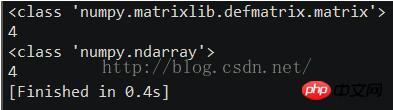
>>> A = arange(12)
>>> A
array([ 0, 1, 2, 3, 4, 5, 6, 7, 8, 9, 10, 11])
>>> A.shape = (3,4)
>>> M = mat(A.copy())
>>> print type(A)," ",type(M)
 
>>> print A
[[ 0 1 2 3]
 [ 4 5 6 7]
 [ 8 9 10 11]]
>>> print M
[[ 0 1 2 3]
 [ 4 5 6 7]
 [ 8 9 10 11]]

现在，让我们简单的切几片。基本的切片使用切片对象或整数。例如，A[:]和M[:]的求值将表现得和Python索引很相似。然而要注意很重要的一点就是NumPy切片数组不创建数据的副本;切片提供统一数据的视图。

>>> print A[:]; print A[:].shape
[[ 0 1 2 3]
 [ 4 5 6 7]
 [ 8 9 10 11]]
(3, 4)
>>> print M[:]; print M[:].shape
[[ 0 1 2 3]
 [ 4 5 6 7]
 [ 8 9 10 11]]
(3, 4)

现在有些和Python索引不同的了：你可以同时使用逗号分割索引来沿着多个轴索引。

>>> print A[:,1]; print A[:,1].shape
[1 5 9]
(3,)
>>> print M[:,1]; print M[:,1].shape
[[1]
 [5]
 [9]]
(3, 1)

注意最后两个结果的不同。对二维数组使用一个冒号产生一个一维数组，然而矩阵产生了一个二维矩阵。10例如，一个M[2,:]切片产生了一个形状为(1,4)的矩阵，相比之下，一个数组的切片总是产生一个最低可能维度11的数组。例如，如果C是一个三维数组，C[...,1]产生一个二维的数组而C[1,:,1]产生一个一维数组。从这时开始，如果相应的矩阵切片结果是相同的话，我们将只展示数组切片的结果。

假如我们想要一个数组的第一列和第三列，一种方法是使用列表切片：

>>> A[:,[1,3]]
array([[ 1, 3],
 [ 5, 7],
 [ 9, 11]])

稍微复杂点的方法是使用take()方法(method):

>>> A[:,].take([1,3],axis=1)
array([[ 1, 3],
 [ 5, 7],
 [ 9, 11]])

如果我们想跳过第一行，我们可以这样：

>>> A[1:,].take([1,3],axis=1)
array([[ 5, 7],
 [ 9, 11]])

或者我们仅仅使用A[1:,[1,3]]。还有一种方法是通过矩阵向量积(叉积)。

>>> A[ix_((1,2),(1,3))]
array([[ 5, 7],
 [ 9, 11]])

为了读者的方便，在次写下之前的矩阵：

>>> A[ix_((1,2),(1,3))]
array([[ 5, 7],
 [ 9, 11]])

现在让我们做些更复杂的。比如说我们想要保留第一行大于1的列。一种方法是创建布尔索引：

>>> A[0,:]>1
array([False, False, True, True], dtype=bool)
>>> A[:,A[0,:]>1]
array([[ 2, 3],
 [ 6, 7],
 [10, 11]])

就是我们想要的！但是索引矩阵没这么方便。

>>> M[0,:]>1
matrix([[False, False, True, True]], dtype=bool)
>>> M[:,M[0,:]>1]
matrix([[2, 3]])

这个过程的问题是用“矩阵切片”来切片产生一个矩阵12，但是矩阵有个方便的A属性，它的值是数组呈现的。所以我们仅仅做以下替代：

>>> M[:,M.A[0,:]>1]
matrix([[ 2, 3],
 [ 6, 7],
 [10, 11]])

如果我们想要在矩阵两个方向有条件地切片，我们必须稍微调整策略，代之以：

>>> A[A[:,0]>2,A[0,:]>1]
array([ 6, 11])
>>> M[M.A[:,0]>2,M.A[0,:]>1]
matrix([[ 6, 11]])

我们需要使用向量积ix_:

>>> A[ix_(A[:,0]>2,A[0,:]>1)]
array([[ 6, 7],
 [10, 11]])
>>> M[ix_(M.A[:,0]>2,M.A[0,:]>1)]
matrix([[ 6, 7],
 [10, 11]])

技巧和提示

下面我们给出简短和有用的提示。

“自动”改变形状

更改数组的维度，你可以省略一个尺寸，它将被自动推导出来。

>>> a = arange(30)
>>> a.shape = 2,-1,3 # -1 means "whatever is needed"
>>> a.shape
(2, 5, 3)
>>> a
array([[[ 0, 1, 2],
 [ 3, 4, 5],
 [ 6, 7, 8],
 [ 9, 10, 11],
 [12, 13, 14]],
 [[15, 16, 17],
 [18, 19, 20],
 [21, 22, 23],
 [24, 25, 26],
 [27, 28, 29]]])

向量组合(stacking)

我们如何用两个相同尺寸的行向量列表构建一个二维数组？在MATLAB中这非常简单：如果x和y是两个相同长度的向量，你仅仅需要做m=[x;y]。在NumPy中这个过程通过函数column_stack、dstack、hstack和vstack来完成，取决于你想要在那个维度上组合。例如：

x = arange(0,10,2)   # x=([0,2,4,6,8])
y = arange(5)    # y=([0,1,2,3,4])
m = vstack([x,y])   # m=([[0,2,4,6,8],
     # [0,1,2,3,4]])
xy = hstack([x,y])   # xy =([0,2,4,6,8,0,1,2,3,4])

二维以上这些函数背后的逻辑会很奇怪。

参考写个Matlab用户的NumPy指南并且在这里添加你的新发现: )

直方图(histogram)

NumPy中histogram函数应用到一个数组返回一对变量：直方图数组和箱式向量。注意：matplotlib也有一个用来建立直方图的函数(叫作hist,正如matlab中一样)与NumPy中的不同。主要的差别是pylab.hist自动绘制直方图，而numpy.histogram仅仅产生数据。

import numpy
import pylab
# Build a vector of 10000 normal deviates with variance 0.5^2 and mean 2
mu, sigma = 2, 0.5
v = numpy.random.normal(mu,sigma,10000)
# Plot a normalized histogram with 50 bins
pylab.hist(v, bins=50, normed=1) # matplotlib version (plot)
pylab.show()
# Compute the histogram with numpy and then plot it
(n, bins) = numpy.histogram(v, bins=50, normed=True) # NumPy version (no plot)
pylab.plot(.5*(bins[1:]+bins[:-1]), n)
pylab.show()

相信看了本文案例你已经掌握了方法，更多精彩请关注php中文网其它相关文章！

推荐阅读：

Pycharm的使用技巧总结

Comment obtenir la valeur maximale locale d'un tableau bidimensionnel en python

Ce qui précède est le contenu détaillé de. pour plus d'informations, suivez d'autres articles connexes sur le site Web de PHP en chinois!