Scikit-Learn による完全な機械学習ワークフロー: カリフォルニアの住宅価格の予測

導入

この記事では、Scikit-Learn を使用した完全な機械学習プロジェクトのワークフローを示します。収入の中央値、住宅築年数、平均部屋数などのさまざまな特徴に基づいて、カリフォルニアの住宅価格を予測するモデルを構築します。このプロジェクトでは、データの読み込み、探索、モデルのトレーニング、評価、結果の視覚化など、プロセスの各ステップをガイドします。基本を理解したい初心者でも、復習を求めている経験豊富な実践者でも、この記事は機械学習テクニックの実際の応用についての貴重な洞察を提供します。

カリフォルニア住宅価格予測プロジェクト

1. はじめに

カリフォルニアの住宅市場は、その独特の特徴と価格動向で知られています。このプロジェクトでは、さまざまな特徴に基づいて住宅価格を予測する機械学習モデルを開発することを目的としています。カリフォルニアの住宅データセットを使用します。これには、収入の中央値、住宅築年数、平均部屋数などのさまざまな属性が含まれます。

2. ライブラリのインポート

このセクションでは、データ操作、視覚化、機械学習モデルの構築に必要なライブラリをインポートします。

import pandas as pd
import matplotlib.pyplot as plt
from sklearn.model_selection import train_test_split
from sklearn.linear_model import LinearRegression
from sklearn.metrics import mean_squared_error
from sklearn.datasets import fetch_california_housing

3. データセットのロード

California Housing データセットをロードし、データを整理するための DataFrame を作成します。ターゲット変数である住宅価格が新しい列として追加されます。

# Load the California Housing dataset
california = fetch_california_housing()
df = pd.DataFrame(california.data, columns=california.feature_names)
df['PRICE'] = california.target

4. サンプルをランダムに選択する

分析を管理しやすくするために、研究用にデータセットから 700 個のサンプルをランダムに選択します。

# Randomly Selecting 700 Samples
df_sample = df.sample(n=700, random_state=42)

5. データを確認する

このセクションでは、データセットの概要を説明し、データの特徴と構造を理解するために最初の 5 行を表示します。

# Overview of the data
print("First five rows of the dataset:")
print(df_sample.head())

出力

First five rows of the dataset:
       MedInc  HouseAge  AveRooms  AveBedrms  Population  AveOccup  Latitude  \
20046  1.6812      25.0  4.192201   1.022284      1392.0  3.877437     36.06   
3024   2.5313      30.0  5.039384   1.193493      1565.0  2.679795     35.14   
15663  3.4801      52.0  3.977155   1.185877      1310.0  1.360332     37.80   
20484  5.7376      17.0  6.163636   1.020202      1705.0  3.444444     34.28   
9814   3.7250      34.0  5.492991   1.028037      1063.0  2.483645     36.62   

       Longitude    PRICE  
20046    -119.01  0.47700  
3024     -119.46  0.45800  
15663    -122.44  5.00001  
20484    -118.72  2.18600  
9814     -121.93  2.78000  

データフレーム情報の表示

print(df_sample.info())

出力

<class 'pandas.core.frame.DataFrame'>
Index: 700 entries, 20046 to 5350
Data columns (total 9 columns):
 #   Column      Non-Null Count  Dtype  
---  ------      --------------  -----  
 0   MedInc      700 non-null    float64
 1   HouseAge    700 non-null    float64
 2   AveRooms    700 non-null    float64
 3   AveBedrms   700 non-null    float64
 4   Population  700 non-null    float64
 5   AveOccup    700 non-null    float64
 6   Latitude    700 non-null    float64
 7   Longitude   700 non-null    float64
 8   PRICE       700 non-null    float64
dtypes: float64(9)
memory usage: 54.7 KB

概要統計の表示

print(df_sample.describe())

出力

           MedInc    HouseAge    AveRooms   AveBedrms   Population  \
count  700.000000  700.000000  700.000000  700.000000   700.000000   
mean     3.937653   28.855714    5.404192    1.079266  1387.422857   
std      2.085831   12.353313    1.848898    0.236318  1027.873659   
min      0.852700    2.000000    2.096692    0.500000     8.000000   
25%      2.576350   18.000000    4.397751    1.005934   781.000000   
50%      3.480000   30.000000    5.145295    1.047086  1159.500000   
75%      4.794625   37.000000    6.098061    1.098656  1666.500000   
max     15.000100   52.000000   36.075472    5.273585  8652.000000   

         AveOccup    Latitude   Longitude       PRICE  
count  700.000000  700.000000  700.000000  700.000000  
mean     2.939913   35.498243 -119.439729    2.082073  
std      0.745525    2.123689    1.956998    1.157855  
min      1.312994   32.590000 -124.150000    0.458000  
25%      2.457560   33.930000 -121.497500    1.218500  
50%      2.834524   34.190000 -118.420000    1.799000  
75%      3.326869   37.592500 -118.007500    2.665500  
max      7.200000   41.790000 -114.590000    5.000010  

6. データセットをトレーニング セットとテスト セットに分割する

データセットを特徴 (X) とターゲット変数 (y) に分割し、モデルのトレーニングと評価のためにトレーニング セットとテスト セットに分割します。

# Splitting the dataset into Train and Test sets
X = df_sample.drop('PRICE', axis=1)  # Features
y = df_sample['PRICE']  # Target variable

# Split the dataset into training and testing sets
X_train, X_test, y_train, y_test = train_test_split(X, y, test_size=0.2, random_state=42)

7. モデルのトレーニング

このセクションでは、トレーニング データを使用して線形回帰モデルを作成およびトレーニングし、特徴と住宅価格の関係を学習します。

# Creating and training the Linear Regression model
lr = LinearRegression()
lr.fit(X_train, y_train)

8. モデルの評価

テスト セットで予測を行い、平均二乗誤差 (MSE) と R 二乗値を計算してモデルのパフォーマンスを評価します。

# Making predictions on the test set
y_pred = lr.predict(X_test)

# Calculating Mean Squared Error
mse = mean_squared_error(y_test, y_pred)
print(f"\nLinear Regression Mean Squared Error: {mse}")

出力

Linear Regression Mean Squared Error: 0.3699851092128846

9. 実際の値と予測値の表示

ここでは、実際の住宅価格とモデルによって生成された予測価格を比較するデータフレームを作成します。

# Displaying Actual vs Predicted Values
results = pd.DataFrame({'Actual Prices': y_test.values, 'Predicted Prices': y_pred})
print("\nActual vs Predicted:")
print(results)

出力

Actual vs Predicted:
     Actual Prices  Predicted Prices
0          0.87500          0.887202
1          1.19400          2.445412
2          5.00001          6.249122
3          2.78700          2.743305
4          1.99300          2.794774
..             ...               ...
135        1.62100          2.246041
136        3.52500          2.626354
137        1.91700          1.899090
138        2.27900          2.731436
139        1.73400          2.017134

[140 rows x

 2 columns]

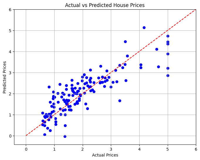
10. 結果の視覚化

最後のセクションでは、散布図を使用して実際の住宅価格と予測住宅価格の関係を視覚化し、モデルのパフォーマンスを視覚的に評価します。

# Visualizing the Results
plt.figure(figsize=(8, 6))
plt.scatter(y_test, y_pred, color='blue')
plt.xlabel('Actual Prices')
plt.ylabel('Predicted Prices')
plt.title('Actual vs Predicted House Prices')

# Draw the ideal line
plt.plot([0, 6], [0, 6], color='red', linestyle='--')

# Set limits to minimize empty space
plt.xlim(y_test.min() - 1, y_test.max() + 1)
plt.ylim(y_test.min() - 1, y_test.max() + 1)

plt.grid()
plt.show()

---

結論

このプロジェクトでは、さまざまな特徴に基づいてカリフォルニアの住宅価格を予測するための線形回帰モデルを開発しました。モデルのパフォーマンスを評価するために平均二乗誤差が計算され、予測精度の定量的な尺度が提供されました。視覚化により、実際の値に対してモデルがどの程度優れたパフォーマンスを発揮するかを確認できました。

このプロジェクトは、不動産分析における機械学習の力を実証し、より高度な予測モデリング技術の基盤として機能します。

以上がScikit-Learn による完全な機械学習ワークフロー: カリフォルニアの住宅価格の予測の詳細内容です。詳細については、PHP 中国語 Web サイトの他の関連記事を参照してください。