

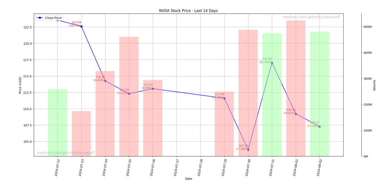
過去 n 日間の株価チャートを生成する Python コード。

コードの各部分の動作について詳しく説明します:
ライブラリのインポート:
matplotlib.pyplot はプロットの作成に使用されます。
yahooquery.Ticker は、Yahoo Finance から過去の株式データを取得するために使用されます。
datetime と timedelta は日付の操作に使用されます。
データ処理には pandas が使用されます。
pytz はタイムゾーンを操作するために使用されます。
os はファイル システムの操作に使用されます。
関数plot_stock_last_n_days:
関数パラメータ:
シンボル: 株式ティッカー (例: 「NVDA」)。
n_days: 履歴データが表示される日数。
filename: プロットが保存されるファイルの名前。
timezone: データを表示するためのタイムゾーン。
日付範囲:
現在の日付と期間の開始日は、n_days に基づいて計算されます。
データの取得:
yahooquery は、指定された期間の過去の株価データを取得するために使用されます。
データの可用性を確認する:
利用可能なデータがない場合は、メッセージが出力され、関数は終了します。
データ処理:
データのインデックスが日時形式に変換され、タイムゾーンが設定されます。
週末 (土曜日と日曜日) は除外されます。
終値の変化率が計算されます。
プロットの作成と構成:
メイン プロットは終値で作成されます。
終値と変化率を示す注釈がプロットに追加されます。
X 軸と Y 軸が構成され、日付がフォーマットされ、グリッド線が追加されます。
取引高の追加プロットが追加され、終値のプラスとマイナスの変化が異なる色で表示されます。
透かしを追加する:
プロットの左下隅と右上隅に透かしが追加されます。
プロットの保存と表示:
プロットは、指定したファイル名で画像ファイルとして保存され、表示されます。
使用例:
この関数はティッカー「NVDA」(NVIDIA) で呼び出され、過去 14 日間のデータを表示し、プロットを「output.png」として保存し、GMT タイムゾーンを使用します。
要約すると、このコードは、終値や取引高などの過去の株価データを、変化率やタイムゾーンの考慮事項の注釈とともに視覚的に表現したものを生成します。
import matplotlib.pyplot as plt
from yahooquery import Ticker
from datetime import datetime, timedelta
import matplotlib.dates as mdates
import os
import pandas as pd
import pytz

def plot_stock_last_n_days(symbol, n_days=30, filename='stock_plot.png', timezone='UTC'):
    # Define the date range
    end_date = datetime.now(pytz.timezone(timezone))
    start_date = end_date - timedelta(days=n_days)

    # Convert dates to the format expected by Yahoo Finance
    start_date_str = start_date.strftime('%Y-%m-%d')
    end_date_str = end_date.strftime('%Y-%m-%d')

    # Fetch historical data for the last n days
    ticker = Ticker(symbol)
    historical_data = ticker.history(start=start_date_str, end=end_date_str, interval='1d')

    # Check if the data is available
    if historical_data.empty:
        print("No data available.")
        return

    # Ensure the index is datetime for proper plotting and localize to the specified timezone
    historical_data.index = pd.to_datetime(historical_data.index.get_level_values('date')).tz_localize('UTC').tz_convert(timezone)

    # Filter out weekends
    historical_data = historical_data[historical_data.index.weekday < 5]

    # Calculate percentage changes
    historical_data['pct_change'] = historical_data['close'].pct_change() * 100

    # Ensure the output directory exists
    output_dir = 'output'
    if not os.path.exists(output_dir):
        os.makedirs(output_dir)

    # Adjust the filename to include the output directory
    filename = os.path.join(output_dir, filename)

    # Plotting the closing price
    fig, ax1 = plt.subplots(figsize=(10, 5))
    ax1.plot(historical_data.index, historical_data['close'], label='Close Price', color='blue', marker='o')

    # Annotate each point with its value and percentage change
    for i in range(1, len(historical_data)):
        date = historical_data.index[i]
        close = historical_data['close'].iloc[i]
        pct_change = historical_data['pct_change'].iloc[i]
        color = 'green' if pct_change > 0 else 'red'
        ax1.text(date, close, f'{close:.2f}\n({pct_change:.2f}%)', fontsize=9, ha='right', color=color)

    # Set up daily gridlines and print date for every day
    ax1.xaxis.set_major_locator(mdates.DayLocator(interval=1))
    ax1.xaxis.set_major_formatter(mdates.DateFormatter('%Y-%m-%d'))

    ax1.set_xlabel('Date')
    ax1.set_ylabel('Price (USD)')
    ax1.set_title(f'{symbol} Stock Price - Last {n_days} Days')
    ax1.legend(loc='upper left')
    ax1.grid(True)
    ax1.tick_params(axis='x', rotation=80)
    fig.tight_layout()

    # Adding the trading volume plot
    ax2 = ax1.twinx()
    calm_green = (0.6, 1, 0.6)  # Calm green color
    calm_red = (1, 0.6, 0.6)    # Calm red color
    colors = [calm_green if historical_data['close'].iloc[i] > historical_data['open'].iloc[i] else calm_red for i in range(len(historical_data))]
    ax2.bar(historical_data.index, historical_data['volume'], color=colors, alpha=0.5, width=0.8)
    ax2.set_ylabel('Volume')
    ax2.tick_params(axis='y')

    # Format y-axis for volume in millions
    def millions(x, pos):
        'The two args are the value and tick position'
        return '%1.0fM' % (x * 1e-6)

    ax2.yaxis.set_major_formatter(plt.FuncFormatter(millions))

    # Adjust the visibility and spacing of the volume axis
    fig.subplots_adjust(right=0.85)
    ax2.spines['right'].set_position(('outward', 60))
    ax2.yaxis.set_label_position('right')
    ax2.yaxis.set_ticks_position('right')

    # Add watermarks
    plt.text(0.01, 0.01, 'medium.com/@dmitry.romanoff', fontsize=12, color='grey', ha='left', va='bottom', alpha=0.5, transform=plt.gca().transAxes)
    plt.text(0.99, 0.99, 'medium.com/@dmitry.romanoff', fontsize=12, color='grey', ha='right', va='top', alpha=0.5, transform=plt.gca().transAxes)

    # Save the plot as an image file
    plt.savefig(filename)
    plt.show()

# Example usage
plot_stock_last_n_days('NVDA', n_days=14, filename='output.png', timezone='GMT')
以上が過去 n 日間の株価チャートを生成する Python コード。の詳細内容です。詳細については、PHP 中国語 Web サイトの他の関連記事を参照してください。

ホットAIツール

Undresser.AI Undress
リアルなヌード写真を作成する AI 搭載アプリ

AI Clothes Remover
写真から衣服を削除するオンライン AI ツール。

Undress AI Tool
脱衣画像を無料で

Clothoff.io
AI衣類リムーバー

Video Face Swap
完全無料の AI 顔交換ツールを使用して、あらゆるビデオの顔を簡単に交換できます。

人気の記事
ホットツール

メモ帳++7.3.1
使いやすく無料のコードエディター

SublimeText3 中国語版
中国語版、とても使いやすい

ゼンドスタジオ 13.0.1
強力な PHP 統合開発環境

ドリームウィーバー CS6
ビジュアル Web 開発ツール

SublimeText3 Mac版
神レベルのコード編集ソフト(SublimeText3)
ホットトピック
 1672
1672
 14
1428
52
1332
25
1277
29
1257
24
14
1428
52
1332
25
1277
29
1257
24

 Python vs. C:曲線と使いやすさの学習
Apr 19, 2025 am 12:20 AM
Python vs. C:曲線と使いやすさの学習
Apr 19, 2025 am 12:20 AM
Pythonは学習と使用が簡単ですが、Cはより強力ですが複雑です。 1。Python構文は簡潔で初心者に適しています。動的なタイピングと自動メモリ管理により、使いやすくなりますが、ランタイムエラーを引き起こす可能性があります。 2.Cは、高性能アプリケーションに適した低レベルの制御と高度な機能を提供しますが、学習しきい値が高く、手動メモリとタイプの安全管理が必要です。
 Pythonの学習:2時間の毎日の研究で十分ですか?
Apr 18, 2025 am 12:22 AM
Pythonの学習:2時間の毎日の研究で十分ですか?
Apr 18, 2025 am 12:22 AM
Pythonを1日2時間学ぶだけで十分ですか?それはあなたの目標と学習方法に依存します。 1)明確な学習計画を策定し、2)適切な学習リソースと方法を選択します。3)実践的な実践とレビューとレビューと統合を練習および統合し、統合すると、この期間中にPythonの基本的な知識と高度な機能を徐々に習得できます。
 Python vs. C:パフォーマンスと効率の探索
Apr 18, 2025 am 12:20 AM
Python vs. C:パフォーマンスと効率の探索
Apr 18, 2025 am 12:20 AM
Pythonは開発効率でCよりも優れていますが、Cは実行パフォーマンスが高くなっています。 1。Pythonの簡潔な構文とリッチライブラリは、開発効率を向上させます。 2.Cのコンピレーションタイプの特性とハードウェア制御により、実行パフォーマンスが向上します。選択を行うときは、プロジェクトのニーズに基づいて開発速度と実行効率を比較検討する必要があります。
 Python vs. C:重要な違いを理解します
Apr 21, 2025 am 12:18 AM
Python vs. C:重要な違いを理解します
Apr 21, 2025 am 12:18 AM
PythonとCにはそれぞれ独自の利点があり、選択はプロジェクトの要件に基づいている必要があります。 1)Pythonは、簡潔な構文と動的タイピングのため、迅速な開発とデータ処理に適しています。 2)Cは、静的なタイピングと手動メモリ管理により、高性能およびシステムプログラミングに適しています。
 Python Standard Libraryの一部はどれですか:リストまたは配列はどれですか?
Apr 27, 2025 am 12:03 AM
Python Standard Libraryの一部はどれですか:リストまたは配列はどれですか?
Apr 27, 2025 am 12:03 AM
PythonListSarePartOfThestAndardarenot.liestareBuilting-in、versatile、forStoringCollectionsのpythonlistarepart。
 Python:自動化、スクリプト、およびタスク管理
Apr 16, 2025 am 12:14 AM
Python:自動化、スクリプト、およびタスク管理
Apr 16, 2025 am 12:14 AM
Pythonは、自動化、スクリプト、およびタスク管理に優れています。 1)自動化:OSやShutilなどの標準ライブラリを介してファイルバックアップが実現されます。 2)スクリプトの書き込み:Psutilライブラリを使用してシステムリソースを監視します。 3)タスク管理:スケジュールライブラリを使用してタスクをスケジュールします。 Pythonの使いやすさと豊富なライブラリサポートにより、これらの分野で優先ツールになります。
 科学コンピューティングのためのPython:詳細な外観
Apr 19, 2025 am 12:15 AM
科学コンピューティングのためのPython:詳細な外観
Apr 19, 2025 am 12:15 AM
科学コンピューティングにおけるPythonのアプリケーションには、データ分析、機械学習、数値シミュレーション、視覚化が含まれます。 1.numpyは、効率的な多次元配列と数学的関数を提供します。 2。ScipyはNumpy機能を拡張し、最適化と線形代数ツールを提供します。 3. Pandasは、データ処理と分析に使用されます。 4.matplotlibは、さまざまなグラフと視覚的な結果を生成するために使用されます。
 Web開発用のPython:主要なアプリケーション
Apr 18, 2025 am 12:20 AM
Web開発用のPython:主要なアプリケーション
Apr 18, 2025 am 12:20 AM
Web開発におけるPythonの主要なアプリケーションには、DjangoおよびFlaskフレームワークの使用、API開発、データ分析と視覚化、機械学習とAI、およびパフォーマンスの最適化が含まれます。 1。DjangoandFlask Framework:Djangoは、複雑な用途の迅速な発展に適しており、Flaskは小規模または高度にカスタマイズされたプロジェクトに適しています。 2。API開発:フラスコまたはdjangorestFrameworkを使用して、Restfulapiを構築します。 3。データ分析と視覚化:Pythonを使用してデータを処理し、Webインターフェイスを介して表示します。 4。機械学習とAI:Pythonは、インテリジェントWebアプリケーションを構築するために使用されます。 5。パフォーマンスの最適化:非同期プログラミング、キャッシュ、コードを通じて最適化
