

ExcelとGoogleシートで色付きのドロップダウンリストを作成する方法

The article shows how to add colors to your data validation lists to make them more visually appealing and user-friendly.
You don't have to be an expert to make a drop-down menu in Excel or Google Sheets. But let's be honest - staring at a long list of values can be pretty boring. If you're looking to add some excitement to your spreadsheets, why not try highlighting a drop-down list with color? Whether you're organizing a list of products, categorizing expenses, or tracking sales data, a colored dropdown will make your data easier to read and understand. In this article, we'll show you how to do just that.

How to create Excel colored drop down list
If you use Excel for data entry, you've likely used the Data Validation feature to create drop-down lists. But did you know that you can also add colors to these lists? This section will guide you through the steps to colorize your drop-down list for a more eye-catching look.
Step 1. Create drop-down list
To add color to your Excel picklist, you first need to create the list itself. If you're unfamiliar with this process, refer to our separate article on creating a drop-down list that describes all possible methods in detail.
For this example, let's assume you have the source list of items in A3:A10 and you've created a drop-down menu with those items. To do that, simply select the range of cells where you want the dropdown to appear (D3:D12 in our case) and click the Data Validation button on the Data tab. In the Data Validation dialog box that appears, choose List from the Allow drop-down menu and, in the Source field, enter the reference to the range of cells containing your items.

Once you've created your drop-down list, you can move on to adding colors.
Step 2. Add colors to drop-down menu
To highlight your picklist with some color, we will be using Excel conditional formatting. The steps are:
- Select the cell(s) with your drop-down menu.
- On the Home tab, in the Styles group, click Conditional Formatting > New Rule… .
- In the New Formatting Rule dialog window, choose the Format only cells that contain option.
- Choose Specific Text from the first drop-down box and containing from the second drop-down box. In the third box, enter the reference to the cell containing the value that you want to format with a certain color like shown in the screenshot below. Alternatively, you can type the value enclosed in double quotes directly in the box, e.g. "Blue".

- Click the Format button.
- In the Format Cells dialog box, switch to the Fill tab, choose the color you like for that particular item, and click OK.
- Back in the New Formatting Rule dialog window, review the settings, and if everything looks good, click OK to save the changes.


Step 3. Test your colored drop-down list
To test your colored drop down menu, click on the arrow next to the cell. You should see the list of items you entered, with the first item highlighted in the chosen color:

Repeat the above steps for other selections and you will get a cohesive color scheme that makes it easy to visually distinguish between different selections.

Tips:
- If you've chosen dark fill colors for your drop-down list, selecting the white font color will make your options more readable. Similarly, if you've chosen light fill colors, using a dark font color will provide better contrast and readability.
- Don't be afraid to experiment with different color combinations to find the one that works best for your data!
- In Excel 365, you can use the brand new IMAGE function to create dropdown with pictures.
How to make Google Sheets drop down list with color
Google Sheets has become a go-to tool for many people. Like its Microsoft Excel counterpart, it offers the ability to create drop-down menus for easier data entry. With the latest version of Google spreadsheets, you no longer need to rely on conditional formatting tricks. Now, you can add colors to your data validation lists directly as you create them!
To create a colored drop-down list in Google Sheets, follow these steps:
- Select one or more cells where we want the dropdown list to appear.
- From the top toolbar, select Data and click Data validation.
- On the Data Validation rules pane, click Add rule.
- In the Criteria drop down menu, pick either the Dropdown or Dropdown from a range option.
- If you choose Dropdown, type your values in the Option 1 and Option 2 boxes, clicking the Add another item button as needed.
If you choose Dropdown from a range, type the range reference in the text field or use the Select Data Range button to pick the range. Either way, be sure to use absolute references with the $ sign to lock cell addresses such as e.g. =$D$4:$D$8.
- Once you've entered your options, it's time to add some color! Simply select the color you want for each item. If you need more tints than shown in the predefined palette, click Customize, and then choose a custom color.
- When you're finished, click the Done button.


There you have it - a colored drop-down menu that not only looks great, but also helps you organize and analyze your data more effectively.

How to create color-coded drop down list
In the first part of this tutorial, you learned how to create dropdown with colored text values. But what if you want to create a color-coded dropdown where only colors are visible, without any text values? This section will show you how to achieve that outcome. By selecting the same color for both the fill and font, you can create a monochromatic effect that is ideal for organizing data in a clear and concise way. Let's dive in and learn how to create a color coded dropdown list with hidden text values.
Color coded dropdown list in Excel
To make a color-coded dropdown in Excel worksheets, you set up conditional formatting rule as described in Adding colors to drop-down menu. When choosing the format, switch between the Fill and Font tabs and pick the same color on both.
Choosing the fill color:

Choosing the font color:

As a result, you will have a color-coded drop down list where each option is represented by a colored cell. This visual representation can be especially useful for data sets with a large number of categories or where color is a significant factor.

Color coded dropdown list in Google Sheets
To color code drop down list in Google Sheets, follow these steps. After adding background colors (Step 6), do the following:
- Click on the color you've added to a certain item, and then click Customize.
- On the Background tab, copy the Hex color code:
- On the Text tab, paste the copied hex code:


That's it! After following the steps outlined above, you'll have a color-coded dropdown menu effectively hiding the text values and leaving only the color swatches visible.

Note. Please remember that the purpose of visual communication is to enhance understanding, and different situations may require different visual cues to achieve that goal. Color codes are useful for representing data where the color is the primary indicator of meaning. However, if you need to provide additional context for each item, using different fill and font colors can be a more effective way to communicate this information visually.
In conclusion, adding color to drop-down lists in Excel and Google Sheets is a great way to enhance the visual appeal of your spreadsheets while also making them more functional and comprehensible. So go ahead and try it out, and see how color can transform your spreadsheets today!
Practice workbook for download
Excel color drop down list (.xlsx file) Google Sheets drop down list with color (online sheet)
以上がExcelとGoogleシートで色付きのドロップダウンリストを作成する方法の詳細内容です。詳細については、PHP 中国語 Web サイトの他の関連記事を参照してください。

ホットAIツール

Undresser.AI Undress
リアルなヌード写真を作成する AI 搭載アプリ

AI Clothes Remover
写真から衣服を削除するオンライン AI ツール。

Undress AI Tool
脱衣画像を無料で

Clothoff.io
AI衣類リムーバー

Video Face Swap
完全無料の AI 顔交換ツールを使用して、あらゆるビデオの顔を簡単に交換できます。

人気の記事
ホットツール

メモ帳++7.3.1
使いやすく無料のコードエディター

SublimeText3 中国語版
中国語版、とても使いやすい

ゼンドスタジオ 13.0.1
強力な PHP 統合開発環境

ドリームウィーバー CS6
ビジュアル Web 開発ツール

SublimeText3 Mac版
神レベルのコード編集ソフト(SublimeText3)
ホットトピック
 7889
7889
 15
1650
14
1411
52
1302
25
1248
29
15
1650
14
1411
52
1302
25
1248
29

 Outlookにカレンダーを追加する方法:共有、インターネットカレンダー、ICALファイル
Apr 03, 2025 am 09:06 AM
Outlookにカレンダーを追加する方法:共有、インターネットカレンダー、ICALファイル
Apr 03, 2025 am 09:06 AM
この記事では、IcalEndarファイルのインポートなど、Outlookデスクトップアプリケーション内で共有カレンダーにアクセスして利用する方法について説明します。 以前は、Outlookカレンダーの共有について説明しました。 それでは、共有されているカレンダーの表示方法を調べてみましょう
 Flash Fill In Excelを使用する方法例
Apr 05, 2025 am 09:15 AM
Flash Fill In Excelを使用する方法例
Apr 05, 2025 am 09:15 AM
このチュートリアルは、データ入力タスクを自動化するための強力なツールであるExcelのFlash Fill機能の包括的なガイドを提供します。 定義と場所から高度な使用やトラブルシューティングまで、さまざまな側面をカバーしています。 ExcelのFLAを理解する
 Excelの式の中央値 - 実用的な例
Apr 11, 2025 pm 12:08 PM
Excelの式の中央値 - 実用的な例
Apr 11, 2025 pm 12:08 PM
このチュートリアルでは、中央値関数を使用してExcelの数値データの中央値を計算する方法について説明します。 中央傾向の重要な尺度である中央値は、データセットの中央値を識別し、中央の傾向のより堅牢な表現を提供します
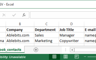 連絡先をOutlookにインポートする方法(CSVおよびPSTファイルから)
Apr 02, 2025 am 09:09 AM
連絡先をOutlookにインポートする方法(CSVおよびPSTファイルから)
Apr 02, 2025 am 09:09 AM
このチュートリアルでは、連絡先をOutlookにインポートするための2つの方法を示しています。CSVファイルとPSTファイルを使用し、オンラインでOutlookに連絡先の転送をカバーしています。 外部ソースからのデータを統合しているかどうか、別のメールプロから移行するかどうか
 Excelでマクロを有効にして無効にする方法
Apr 02, 2025 am 09:05 AM
Excelでマクロを有効にして無効にする方法
Apr 02, 2025 am 09:05 AM
この記事では、マクロセキュリティの基本と安全なVBAコードの実行をカバーして、Excelでマクロを有効にする方法について説明します。 マクロは、あらゆる技術と同様に、二重の可能性、つまり最新の自動化または悪意のある使用です。 Excelのデフォルト設定は、SAのマクロを無効にします
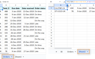
 Googleシートクエリ機能の使用方法 - 標準条項と代替ツール
Apr 02, 2025 am 09:21 AM
Googleシートクエリ機能の使用方法 - 標準条項と代替ツール
Apr 02, 2025 am 09:21 AM
この包括的なガイドは、Googleシートのクエリ関数のパワーを解き放ち、しばしば最も強力なスプレッドシート関数として歓迎されます。 その構文を分析し、さまざまな条項を調査してデータ操作をマスターします。 Googleシートを理解する
 Excel共有ワークブック:複数のユーザーのExcelファイルを共有する方法
Apr 11, 2025 am 11:58 AM
Excel共有ワークブック:複数のユーザーのExcelファイルを共有する方法
Apr 11, 2025 am 11:58 AM
このチュートリアルは、さまざまな方法、アクセス制御、競合解決をカバーするExcelワークブックを共有するための包括的なガイドを提供します。 Modern Excelバージョン(2010、2013、2016、およびその後)共同編集を簡素化し、mの必要性を排除します
 Googleシートフィルター機能の使用方法
Apr 02, 2025 am 09:19 AM
Googleシートフィルター機能の使用方法
Apr 02, 2025 am 09:19 AM
Googleシートのフィルター機能のパワーのロックを解除:包括的なガイド 基本的なGoogleシートフィルタリングにうんざりしていませんか? このガイドは、フィルター関数の機能を発表し、標準フィルタリングツールの強力な代替品を提供します。私たちはexploします
