여러 기준으로 Excel Xlookup

The tutorial shows how to use Excel XLOOKUP with multiple criteria and explains the advantages and limitations of this method.

In Excel, there's this awesome function called XLOOKUP, which makes it really easy to find specific values in your tables. And guess what? It doesn't just look for one thing, it can also search using different conditions. In this article, we'll show you how to combine different criteria to find the perfect match for your data. You'll be amazed by how much you can do with this function!

• XLOOKUP formula with multiple criteria
• How to use XLOOKUP multiple criteria
• Multiple criteria XLOOKUP with logical operators
• Multiple criteria XLOOKUP approximate match
• XLOOKUP formula with multiple OR conditions
• XLOOKUP with AND and OR conditions
• Advantages and limitations

Excel XLOOKUP with multiple criteria

Before delving into multiple criteria, let's quickly go over the XLOOKUP syntax, focusing on the essentials:

XLOOKUP(lookup_value, lookup_array, return_array, [if_not_found], [match_mode], [search_mode])

For our purposes, we're particularly interested in the first three arguments:

• lookup_value - the value you're searching for.
• lookup_array - the range where you want to search for the lookup value.
• return_array - the range from which to return the corresponding value.

For a deeper understanding, you can explore more details in the article: Excel XLOOKUP function - syntax and uses.

While XLOOKUP is designed to handle just one lookup value, we've got tricks up our sleeves to overcome this limitation :)

Formula 1. Boolean logic

The easiest way to use XLOOKUP with multiple criteria is to apply the Boolean logic. This term simply says things are either true or false. In our XLOOKUP, this means:

XLOOKUP(1, (lookup_array1 = lookup_value1) * (lookup_array2 = lookup_value2) * (…), return_array)

Here's the scoop: XLOOKUP hunts for the number 1 while creating a temporary lookup array filled with 0’s (no match) and 1’s (match). First, you check each lookup value against all values in the corresponding lookup array, creating an array of TRUE and FALSE values. And then, you multiply these arrays, turning TRUE and FALSE into 1 and 0 and forming a single lookup array. This final array has 1 for the items meeting all criteria, and XLOOKUP returns the first found match.

For example, to find the supplier of the target item in the target region, the generic formula would be:

=XLOOKUP(1, (Items=Target_Item) * (Regions=Target_Region), Suppliers)

Formula 2. Concatenation

Another approach involves combining all the target values (conditions) into a single lookup_value using the concatenation operator (&). Then, search for that value in the concatenated lookup_array:

XLOOKUP(lookup_value1 & lookup_value2 & …, lookup_array1 & lookup_array2 & …, return_array)

For instance, to get the supplier of a particular product based on its name and region, you can use the formula:

=XLOOKUP(Target_Item & Target_Region , Items & Regions, Suppliers)

While this formula shines in simplicity, it might stumble in more complex scenarios, especially when dealing with logical operators or OR logic. Therefore, we recommend the Boolean logic approach for its versatility and reliability.

Tip. If you are using an older version of Excel without the XLOOKUP function, you can achieve the same magic with the trusty INDEX MATCH formula with multiple criteria.

How to use XLOOKUP with multiple criteria

Now that we've covered the basic formula, let's dive into the practical application. Imagine your quest is to find the supplier based on three criteria: item name, region, and delivery type. The task can be accomplished with two different formulas detailed below. While both formulas lead to the same result, they take different routes.

Multiple criteria XLOOKUP formula: Boolean logic

For our sample dataset, use the following formula to get the supplier based on 3 criteria in cells G4, G5 and G6:

=XLOOKUP(1, (A3:A22=G4) * (B3:B22=G5) * (C3:C22=G6), D3:D22)

Here's a breakdown of how this formula works:

1. Testing individual conditions First, the formula compares the target item in cell G4 against all items in the range A3:A22. Similarly, it checks the region in G5 against all regions in B3:B22 and the delivery type in G6 against all delivery services in C3:C22. These comparisons generate three arrays of TRUE and FALSE values like this:

   {FALSE;FALSE;FALSE;FALSE;FALSE;FALSE;TRUE;TRUE;TRUE;…} * {FALSE;FALSE;FALSE;TRUE;TRUE;TRUE;FALSE;FALSE;TRUE;… } * {FALSE;TRUE;FALSE;FALSE;TRUE;FALSE;FALSE;TRUE;FALSE;…}

2. Multiplication operation The multiplication operation converts TRUE and FALSE values to 1’s and 0’s, respectively, forming a single lookup array. Multiplying by 0 ensures only items meeting all the criteria are represented by 1.

   {0;0;0;0;0;0;0;0;0;1;0;0;0;0;0;0;0;0;0;0}

3. XLOOKUP in action This array becomes the lookup_array for XLOOKUP, where it’s searching for the number 1. The 10th value in the array being 1 corresponds to the 10th entry in the dataset. XLOOKUP finds it and returns the 10th value in the return_array (D3:D22), which is "Elijah."

XLOOKUP formula with multiple criteria: concatenation

The same task can be accomplished with this formula:

=XLOOKUP(G4 & G5 & G6, A3:A22 & B3:B22 & C3:C22, D3:D22)

Here's the breakdown for this approach:

1. Concatenating lookup values Concatenate all three lookup values (G4, G5, and G6) into a single lookup_value using the concatenation operator. In simple terms, we're creating a combined string to look for: "OrangesWestExpedited".
2. Concatenating lookup arrays Concatenate the respective ranges A3:A22, B3:B22, and C3:C22 to create a single lookup_array such as:

   {"ApplesEastStandard";"ApplesEastExpedited";"ApplesEastOvernight";"ApplesWestStandard";"ApplesWestExpedited";"ApplesWestOvernight";"OrangesEastStandard";"OrangesEastExpedited";"OrangesWestStandard";"OrangesWestExpedited"; …}

3. XLOOKUP at your service XLOOKUP searches for the concatenated lookup value in the combined lookup array. When it identifies the matching row, it returns the corresponding value from the return array (D3:D22).

Tip. To gain insights into your Excel formulas, you can use F9 key for formula evaluation and see all the intermediate results in the formula bar.

Multiple criteria XLOOKUP with logical operators

Expanding the horizon of multiple criteria XLOOKUP, you can go beyond simple equality checks by incorporating various logical operators. These operators allow you to test conditions such as greater than, less than, or not equal to specific values.

For instance, consider the scenario of getting the supplier for the item in G4, the region not matching G5, and a discount greater than G6. The formula to achieve this is as follows:

=XLOOKUP(1, (A3:A22=G4) * (B3:B22<>G5) * (C3:C22>G6), D3:D22)

Multiple criteria XLOOKUP approximate match

The basic XLOOKUP formula can seek an exact or approximate match, controlled by the 5th argument, match_mode. When dealing with multiple conditions, the challenge arises in finding a value that approximately matches one of the criteria.

The solution involves first filtering out entries that don't meet the exact match condition, achieved through the IF or FILTER function. The filtered array is then served to XLOOKUP, prompting an approximate match - you choose between the closest smaller item (match_mode set to -1) or the closest larger one (match_mode set to 1).

In an example scenario with item names in column A, quantities in column B, and discounts in column C, aiming to find the discount for a specific item in cell F4 and a quantity in F5, the formula is constructed as follows:

=XLOOKUP(F5, IF(A3:A22=F4, B3:B22), C3:C22,, -1)

Breaking it down, the inner logic filters items matching F4 and their corresponding quantities:

IF(A3:A22=F4, B3:B22)

This results in an array consisting of quantity numbers for matching items and FALSE for non-matching ones:

{…;FALSE;FALSE;FALSE;20;50;100;150;200;250;FALSE;FALSE;FALSE;…}

With the target quantity of 75 in F5, XLOOKUP with match_mode set to -1, searches for the next smaller item in the above array, finds 50, and returns the corresponding discount from column C (3%).

Alternatively, you can do filtering using the FILTER function:

=XLOOKUP(F5, FILTER(B3:B22, A3:A22=F4), FILTER(C3:C22, A3:A22=F4),, -1)

In this version, you filter quantities (B3:B22) based on the target item (A3:A22=F4) for the lookup array, and for the return array, you filter discounts (C3:C22) for the same target item.

XLOOKUP with multiple conditions (OR logic)

In our previous examples, we delved into AND logic, finding the value that meets all of the specified criteria. Now, let's explore how to use XLOOKUP with OR logic, finding values that meet at least one of the conditions.

Depending on whether your criteria are in the same column or in different columns, there are 2 variations of the formula.

XLOOKUP formula for multiple OR criteria in the same column

This formula employs Boolean logic with the addition operation (+) representing OR logic:

XLOOKUP(1, (lookup_array = lookup_value1) + (lookup_array = lookup_value2) + (…), return_array)

In simple terms, when you multiply arrays of TRUE and FALSE values from individual criteria tests, multiplying by 0 ensures that only items meeting all the criteria end up with the number 1 in the final lookup array (AND logic). On the other hand, using the addition operation ensures that items meeting any single criteria are represented by 1 (OR logic). As a result, an XLOOKUP formula with the lookup value set to 1 effectively fetches the value for which any condition is true.

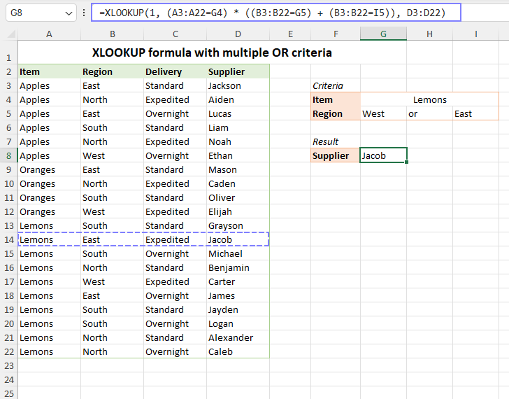
For example, to retrieve the first record in the below dataset where the region is either G4 or I4, the formula is:

=XLOOKUP(1, (B3:B22=G4) + (B3:B22=I4), A3:D22)

Note. If there are two or more entries matching any of the conditions, the formula returns the first found match.

XLOOKUP formula for multiple OR criteria in different columns

When dealing with several OR criteria in a single column, the test results are clear-cut - only one test can return TRUE. This simplicity allows adding up the elements of the resulting arrays, yielding a final array with only 0s (none of the criteria is true) and 1s (one of the criteria is true), perfectly aligning with the lookup value 1.

However, when testing multiple columns, things get trickier. The tests are not mutually exclusive as more than one column can meet the criteria, resulting in more than one logical test returning TRUE. Consequently, the final array may contain values greater than 1.

To address this, adjust the formula as follows:

XLOOKUP(1, --((lookup_array1 =lookup_value1) + (lookup_array2 =lookup_value2) + (…) > 0), return_array)

In this adaptation, you add up the intermediate arrays, and then check if the values in the resulting array are greater than 0. This gives us a new array comprised of only TRUE and FALSE values. The double negation (--) changes these TRUEs and FALSEs into 1s and 0s, making sure our lookup value of 1 still does its job smoothly.

For example, to fetch the first record from A3:B22 that has “Yes” in either column C or D, or in both columns, you can use a formula like this:

=XLOOKUP(1, --((C3:C22 = "Yes") + (D3:D22 = "Yes") >0), A3:B22)

Naturally, you are free to adjust the logic as needed to target your desired data.

Complex scenario: combining AND and OR logic

In more complex cases, you might need a combination of AND as well as OR logic. For example, to get the supplier for the item in G4 and the region either in G5 or I5, use this formula:

=XLOOKUP(1, (A3:A22=G4) * ((B3:B22=G5) + (B3:B22=I5)), D3:D22)

Where:

• (A3:A22=G4) checks if the item in the lookup range matches the target item name in cell G4.
• ((B3:B22=G5) + (B3:B22=I5)) implements OR logic by checking if the region is either G5 or I5.
• (A3:A22=G4) * ((B3:B22=G5) + (B3:B22=I5)) implements AND logic for the item name and region.
• D3:D22 returns the corresponding supplier from this range.

The overall formula successfully locates the first match where both the item and region criteria are met, applying AND and OR logic to different criteria.

Advantages and limitations of multiple criteria XLOOKUP

Using XLOOKUP with multiple criteria offers both advantages and limitations worth considering.

Advantages

The benefits of the multiple criteria XLOOKUP are:

• Find specific details easily. With XLOOKUP, it's easier to find exactly what you're looking for in your data, especially when you have more than one condition. This means you can be very specific about the information you want to retrieve.
• Flexibility in criteria. You can use as many conditions as you need. Just make sure that all the lookup arrays are the same size.
• Dynamic arrays. You can use XLOOKUP with dynamic arrays, which means that you can spill the results to multiple cells without using old-fashioned Ctrl + Shift + Enter array formulas.
• Easy to understand. XLOOKUP formulas are written in a way that's easy to read and understand. This is helpful not only for you but also for others who might work with your Excel sheets.

Limitations

The limitations of XLOOKUP with the multiple criteria are:

• Unique criteria combinations. You need to have a unique combination of conditions for your lookup values, otherwise XLOOKUP will return an error or the first match.
• Consistent array dimensions. The lookup and return arrays must have the same number of rows or columns. A mismatch in dimensions will result in an error.

To sum up, you can do amazing things with data analysis by using Excel's XLOOKUP function with multiple criteria. It allows you to search for exactly what you need, making your work more organized and efficient. The key is to make sure that each item you want to find has a unique combination of criteria, and that all the data you're searching through is arranged consistently. So, go ahead, try these tips and make your Excel tasks more productive and enjoyable!

Practice workbook for download

Multiple criteria XLOOKUP – formula examples (.xlsx file)

위 내용은 여러 기준으로 Excel Xlookup의 상세 내용입니다. 자세한 내용은 PHP 중국어 웹사이트의 기타 관련 기사를 참조하세요!