TensorFlow를 사용한 올가미 회귀 및 능선 회귀 알고리즘 구현 예

이 글에서는 TensorFlow를 사용하여 Lasso 회귀 및 능선 회귀 알고리즘을 구현하는 예를 주로 소개합니다. 이제는 필요한 친구들이 참조할 수 있도록 공유합니다.

또한 제한할 수 있는 몇 가지 방법이 있습니다. 회귀 알고리즘의 출력 결과 가장 일반적으로 사용되는 두 가지 정규화 방법은 올가미 회귀와 능선 회귀입니다.

올가미 회귀 및 능선 회귀 알고리즘은 기존 선형 회귀 알고리즘과 매우 유사합니다. 한 가지 차이점은 기울기(또는 순 기울기)를 제한하기 위해 공식에 정규 항이 추가된다는 것입니다. 이렇게 하는 주된 이유는 기울기 A에 따라 달라지는 손실 함수를 추가하여 종속 변수에 대한 특성의 영향을 제한하는 것입니다.

올가미 회귀 알고리즘의 경우 손실 함수에 기울기 A의 주어진 배수 항목을 추가합니다. 우리는 TensorFlow의 논리 연산을 사용하지만 이러한 연산과 관련된 기울기 없이 대신 컷오프 지점에서 점프하고 확장하는 연속 계단 함수라고도 하는 계단 함수의 연속 추정을 사용합니다. 잠시 후 올가미 회귀 알고리즘을 사용하는 방법을 살펴보겠습니다.

능선 회귀 알고리즘의 경우 경사 계수의 L2 정규화인 L2 표준을 추가합니다.

# LASSO and Ridge Regression
# lasso回归和岭回归
# 
# This function shows how to use TensorFlow to solve LASSO or 
# Ridge regression for 
# y = Ax + b
# 
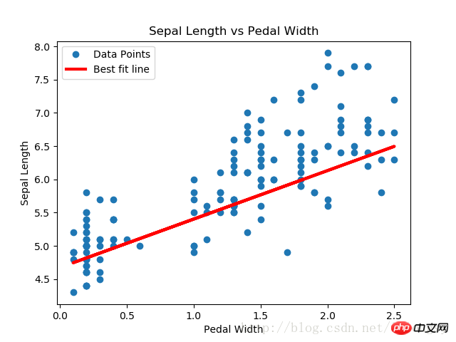
# We will use the iris data, specifically: 
#  y = Sepal Length 
#  x = Petal Width

# import required libraries
import matplotlib.pyplot as plt
import sys
import numpy as np
import tensorflow as tf
from sklearn import datasets
from tensorflow.python.framework import ops


# Specify 'Ridge' or 'LASSO'
regression_type = 'LASSO'

# clear out old graph
ops.reset_default_graph()

# Create graph
sess = tf.Session()

###
# Load iris data
###

# iris.data = [(Sepal Length, Sepal Width, Petal Length, Petal Width)]
iris = datasets.load_iris()
x_vals = np.array([x[3] for x in iris.data])
y_vals = np.array([y[0] for y in iris.data])

###
# Model Parameters
###

# Declare batch size
batch_size = 50

# Initialize placeholders
x_data = tf.placeholder(shape=[None, 1], dtype=tf.float32)
y_target = tf.placeholder(shape=[None, 1], dtype=tf.float32)

# make results reproducible
seed = 13
np.random.seed(seed)
tf.set_random_seed(seed)

# Create variables for linear regression
A = tf.Variable(tf.random_normal(shape=[1,1]))
b = tf.Variable(tf.random_normal(shape=[1,1]))

# Declare model operations
model_output = tf.add(tf.matmul(x_data, A), b)

###
# Loss Functions
###

# Select appropriate loss function based on regression type

if regression_type == 'LASSO':
  # Declare Lasso loss function
  # 增加损失函数，其为改良过的连续阶跃函数，lasso回归的截止点设为0.9。
  # 这意味着限制斜率系数不超过0.9
  # Lasso Loss = L2_Loss + heavyside_step,
  # Where heavyside_step ~ 0 if A < constant, otherwise ~ 99
  lasso_param = tf.constant(0.9)
  heavyside_step = tf.truep(1., tf.add(1., tf.exp(tf.multiply(-50., tf.subtract(A, lasso_param)))))
  regularization_param = tf.multiply(heavyside_step, 99.)
  loss = tf.add(tf.reduce_mean(tf.square(y_target - model_output)), regularization_param)

elif regression_type == &#39;Ridge&#39;:
  # Declare the Ridge loss function
  # Ridge loss = L2_loss + L2 norm of slope
  ridge_param = tf.constant(1.)
  ridge_loss = tf.reduce_mean(tf.square(A))
  loss = tf.expand_dims(tf.add(tf.reduce_mean(tf.square(y_target - model_output)), tf.multiply(ridge_param, ridge_loss)), 0)

else:
  print(&#39;Invalid regression_type parameter value&#39;,file=sys.stderr)


###
# Optimizer
###

# Declare optimizer
my_opt = tf.train.GradientDescentOptimizer(0.001)
train_step = my_opt.minimize(loss)

###
# Run regression
###

# Initialize variables
init = tf.global_variables_initializer()
sess.run(init)

# Training loop
loss_vec = []
for i in range(1500):
  rand_index = np.random.choice(len(x_vals), size=batch_size)
  rand_x = np.transpose([x_vals[rand_index]])
  rand_y = np.transpose([y_vals[rand_index]])
  sess.run(train_step, feed_dict={x_data: rand_x, y_target: rand_y})
  temp_loss = sess.run(loss, feed_dict={x_data: rand_x, y_target: rand_y})
  loss_vec.append(temp_loss[0])
  if (i+1)%300==0:
    print(&#39;Step #&#39; + str(i+1) + &#39; A = &#39; + str(sess.run(A)) + &#39; b = &#39; + str(sess.run(b)))
    print(&#39;Loss = &#39; + str(temp_loss))
    print(&#39;\n&#39;)

###
# Extract regression results
###

# Get the optimal coefficients
[slope] = sess.run(A)
[y_intercept] = sess.run(b)

# Get best fit line
best_fit = []
for i in x_vals:
 best_fit.append(slope*i+y_intercept)


###
# Plot results
###

# Plot regression line against data points
plt.plot(x_vals, y_vals, &#39;o&#39;, label=&#39;Data Points&#39;)
plt.plot(x_vals, best_fit, &#39;r-&#39;, label=&#39;Best fit line&#39;, linewidth=3)
plt.legend(loc=&#39;upper left&#39;)
plt.title(&#39;Sepal Length vs Pedal Width&#39;)
plt.xlabel(&#39;Pedal Width&#39;)
plt.ylabel(&#39;Sepal Length&#39;)
plt.show()

# Plot loss over time
plt.plot(loss_vec, &#39;k-&#39;)
plt.title(regression_type + &#39; Loss per Generation&#39;)
plt.xlabel(&#39;Generation&#39;)
plt.ylabel(&#39;Loss&#39;)
plt.show()

출력 결과:

단계 #300 A = [[ 0.77170753]] b = [[ 1.82499862]]
손실 = [[ 10.26473045]]
단계 #600 A = [[ 0 .7 5908542]] b = [[ 3.2220633]]
손실 = [[ 3.06292033]]
단계 #900 A = [[ 0.74843585]] b = [[ 3.9975822]]
손실 = [[ 1.23220456]]
단계 #1200 A = [[ 0.73 7 52165] ] b = [[ 4.42974091]]
손실 = [[ 0.57872057]]
단계 #1500 A = [[ 0.72942668]] b = [[ 4.67253113]]
손실 = [[ 0.40874988]]

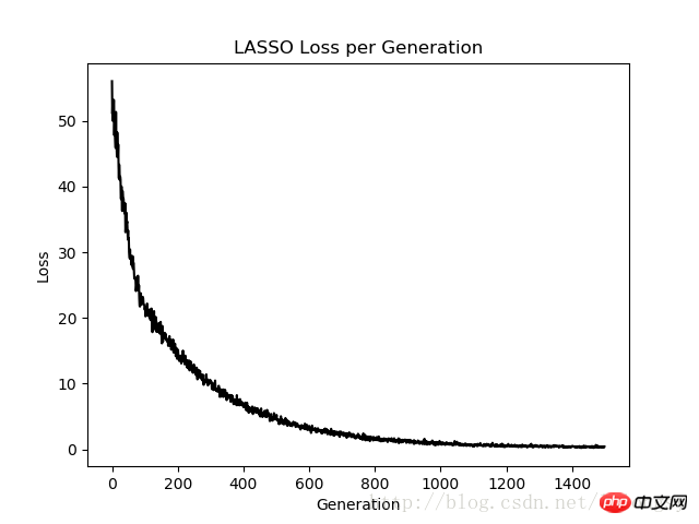
라쏘 회귀 알고리즘은 표준 선형 회귀 추정을 기반으로 연속 계단 함수를 추가하여 구현됩니다. 스텝 함수의 기울기로 인해 스텝 크기에 주의해야 합니다. 스텝 크기가 너무 크면 결국 수렴되지 않는 결과를 낳기 때문입니다.

관련 권장 사항:

TensorFlow

을 사용하여 Deming 회귀 알고리즘을 구현하는 예

위 내용은 TensorFlow를 사용한 올가미 회귀 및 능선 회귀 알고리즘 구현 예의 상세 내용입니다. 자세한 내용은 PHP 중국어 웹사이트의 기타 관련 기사를 참조하세요!