Cara membuat jadual kandungan dinamik di Excel

A table of contents is a total game-changer when working with large files – it keeps everything organized and easy to navigate. Unfortunately, unlike Word, Microsoft Excel doesn’t have a simple “Table of Contents” button that adds this handy feature and updates it automatically. No, you’ll have to roll up your sleeves and create a dynamic table of contents yourself. This table will automatically update and contain clickable links, allowing you to add and remove sheets – as well as jump between them – with ease. This guide has all the info you need to create a dynamic table of contents in Excel.

How to Create a Dynamic Table of Contents in Excel

Technically, there are three ways to create a dynamic table of contents (TOC) in Excel. However, only one of them guarantees a fully automated TOC, and that’s Visual Basic for Applications or VBA for short – Microsoft’s native programming language. The other two – traditional formulas and Power Query – will give you a semi-dynamic table of contents in Excel – one that either doesn’t include clickable links or doesn’t update automatically. Since we’re after a fully dynamic Excel table of contents, we’ll use VBA.

If you aren’t particularly VBA-savvy; don’t worry – you just need to follow a few steps. But first – let’s create our table of contents.

Step 1: Click on the “Insert Worksheet” button next to your sheets at the bottom.

Step 2: Name the sheet “Table of Contents.”

Step 3: Drag the sheet to the first position for better navigation.

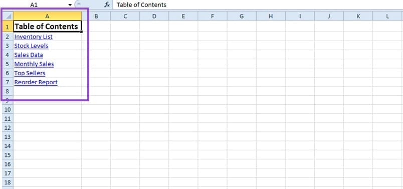
Step 4: Enter the names of your sheets in Column A of the “Table of Contents” sheet.

And voilà – you’ve got your table of contents. You can play with the aesthetics of this TOC later – now, we need to make it dynamic. To do so, we’ll need the help of the VBA Editor – a built-in Excel tool that lets you write and run custom codes.

Step 1: Press “Alt + F11” to open the VBA Editor.

Step 2: Go to the “Insert” tab at the top.

Step 3: Select “Module” from the dropdown menu.

Step 4: Copy and paste the following VBA code:

Sub CreateTOC()

    Dim ws As Worksheet

    Dim toc As Worksheet

    Dim i As Integer

    ‘ Check if TOC sheet already exists, delete if it does

    On Error Resume Next

    Set toc = ThisWorkbook.Sheets(“Table of Contents”)

    On Error GoTo 0

    If Not toc Is Nothing Then Application.DisplayAlerts = False: toc.Delete: Application.DisplayAlerts = True

    ‘ Create new TOC sheet

    Set toc = ThisWorkbook.Sheets.Add(Before:=ThisWorkbook.Sheets(1))

    toc.Name = “Table of Contents”

    ‘ Set up TOC header

    toc.Cells(1, 1).Value = “Table of Contents”

    toc.Cells(1, 1).Font.Bold = True

    toc.Cells(1, 1).Font.Size = 14

    ‘ Loop through all sheets and add hyperlinks

    i = 2

    For Each ws In ThisWorkbook.Sheets

        If ws.Name <> “Table of Contents” Then

            toc.Hyperlinks.Add Anchor:=toc.Cells(i, 1), _

                Address:=””, _

                SubAddress:=”‘” & ws.Name & “‘!A1”, _

                TextToDisplay:=ws.Name

            i = i + 1

        End If

    Next ws

    ‘ Adjust column width

    toc.Columns(“A”).AutoFit

 End Sub

Step 5: Hit “F5” to run the code.

Step 6: Exit the VBA Editor.

You’ll notice your Excel table of contents is now clickable.

To automatically update your table of contents after changes, you just need to repeat Steps 1 to 6. This will add any new sheets to the list or remove the ones you deleted.

Atas ialah kandungan terperinci Cara membuat jadual kandungan dinamik di Excel. Untuk maklumat lanjut, sila ikut artikel berkaitan lain di laman web China PHP!