

Cara Membuat Senarai Drop Down Berwarna Dalam Lembaran Excel dan Google

The article shows how to add colors to your data validation lists to make them more visually appealing and user-friendly.
You don't have to be an expert to make a drop-down menu in Excel or Google Sheets. But let's be honest - staring at a long list of values can be pretty boring. If you're looking to add some excitement to your spreadsheets, why not try highlighting a drop-down list with color? Whether you're organizing a list of products, categorizing expenses, or tracking sales data, a colored dropdown will make your data easier to read and understand. In this article, we'll show you how to do just that.

How to create Excel colored drop down list
If you use Excel for data entry, you've likely used the Data Validation feature to create drop-down lists. But did you know that you can also add colors to these lists? This section will guide you through the steps to colorize your drop-down list for a more eye-catching look.
Step 1. Create drop-down list
To add color to your Excel picklist, you first need to create the list itself. If you're unfamiliar with this process, refer to our separate article on creating a drop-down list that describes all possible methods in detail.
For this example, let's assume you have the source list of items in A3:A10 and you've created a drop-down menu with those items. To do that, simply select the range of cells where you want the dropdown to appear (D3:D12 in our case) and click the Data Validation button on the Data tab. In the Data Validation dialog box that appears, choose List from the Allow drop-down menu and, in the Source field, enter the reference to the range of cells containing your items.

Once you've created your drop-down list, you can move on to adding colors.
Step 2. Add colors to drop-down menu
To highlight your picklist with some color, we will be using Excel conditional formatting. The steps are:
- Select the cell(s) with your drop-down menu.
- On the Home tab, in the Styles group, click Conditional Formatting > New Rule… .
- In the New Formatting Rule dialog window, choose the Format only cells that contain option.
- Choose Specific Text from the first drop-down box and containing from the second drop-down box. In the third box, enter the reference to the cell containing the value that you want to format with a certain color like shown in the screenshot below. Alternatively, you can type the value enclosed in double quotes directly in the box, e.g. "Blue".

- Click the Format button.
- In the Format Cells dialog box, switch to the Fill tab, choose the color you like for that particular item, and click OK.
- Back in the New Formatting Rule dialog window, review the settings, and if everything looks good, click OK to save the changes.


Step 3. Test your colored drop-down list
To test your colored drop down menu, click on the arrow next to the cell. You should see the list of items you entered, with the first item highlighted in the chosen color:

Repeat the above steps for other selections and you will get a cohesive color scheme that makes it easy to visually distinguish between different selections.

Tips:
- If you've chosen dark fill colors for your drop-down list, selecting the white font color will make your options more readable. Similarly, if you've chosen light fill colors, using a dark font color will provide better contrast and readability.
- Don't be afraid to experiment with different color combinations to find the one that works best for your data!
- In Excel 365, you can use the brand new IMAGE function to create dropdown with pictures.
How to make Google Sheets drop down list with color
Google Sheets has become a go-to tool for many people. Like its Microsoft Excel counterpart, it offers the ability to create drop-down menus for easier data entry. With the latest version of Google spreadsheets, you no longer need to rely on conditional formatting tricks. Now, you can add colors to your data validation lists directly as you create them!
To create a colored drop-down list in Google Sheets, follow these steps:
- Select one or more cells where we want the dropdown list to appear.
- From the top toolbar, select Data and click Data validation.
- On the Data Validation rules pane, click Add rule.
- In the Criteria drop down menu, pick either the Dropdown or Dropdown from a range option.
- If you choose Dropdown, type your values in the Option 1 and Option 2 boxes, clicking the Add another item button as needed.
If you choose Dropdown from a range, type the range reference in the text field or use the Select Data Range button to pick the range. Either way, be sure to use absolute references with the $ sign to lock cell addresses such as e.g. =$D$4:$D$8.
- Once you've entered your options, it's time to add some color! Simply select the color you want for each item. If you need more tints than shown in the predefined palette, click Customize, and then choose a custom color.
- When you're finished, click the Done button.


There you have it - a colored drop-down menu that not only looks great, but also helps you organize and analyze your data more effectively.

How to create color-coded drop down list
In the first part of this tutorial, you learned how to create dropdown with colored text values. But what if you want to create a color-coded dropdown where only colors are visible, without any text values? This section will show you how to achieve that outcome. By selecting the same color for both the fill and font, you can create a monochromatic effect that is ideal for organizing data in a clear and concise way. Let's dive in and learn how to create a color coded dropdown list with hidden text values.
Color coded dropdown list in Excel
To make a color-coded dropdown in Excel worksheets, you set up conditional formatting rule as described in Adding colors to drop-down menu. When choosing the format, switch between the Fill and Font tabs and pick the same color on both.
Choosing the fill color:

Choosing the font color:

As a result, you will have a color-coded drop down list where each option is represented by a colored cell. This visual representation can be especially useful for data sets with a large number of categories or where color is a significant factor.

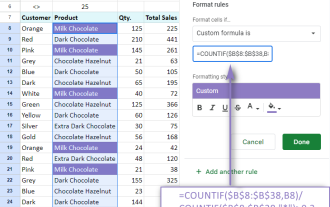
Color coded dropdown list in Google Sheets
To color code drop down list in Google Sheets, follow these steps. After adding background colors (Step 6), do the following:
- Click on the color you've added to a certain item, and then click Customize.
- On the Background tab, copy the Hex color code:
- On the Text tab, paste the copied hex code:


That's it! After following the steps outlined above, you'll have a color-coded dropdown menu effectively hiding the text values and leaving only the color swatches visible.

Note. Please remember that the purpose of visual communication is to enhance understanding, and different situations may require different visual cues to achieve that goal. Color codes are useful for representing data where the color is the primary indicator of meaning. However, if you need to provide additional context for each item, using different fill and font colors can be a more effective way to communicate this information visually.
In conclusion, adding color to drop-down lists in Excel and Google Sheets is a great way to enhance the visual appeal of your spreadsheets while also making them more functional and comprehensible. So go ahead and try it out, and see how color can transform your spreadsheets today!
Practice workbook for download
Excel color drop down list (.xlsx file) Google Sheets drop down list with color (online sheet)
Atas ialah kandungan terperinci Cara Membuat Senarai Drop Down Berwarna Dalam Lembaran Excel dan Google. Untuk maklumat lanjut, sila ikut artikel berkaitan lain di laman web China PHP!

Alat AI Hot

Undresser.AI Undress
Apl berkuasa AI untuk mencipta foto bogel yang realistik

AI Clothes Remover
Alat AI dalam talian untuk mengeluarkan pakaian daripada foto.

Undress AI Tool
Gambar buka pakaian secara percuma

Clothoff.io
Penyingkiran pakaian AI

Video Face Swap
Tukar muka dalam mana-mana video dengan mudah menggunakan alat tukar muka AI percuma kami!

Artikel Panas
Alat panas

Notepad++7.3.1
Editor kod yang mudah digunakan dan percuma

SublimeText3 versi Cina
Versi Cina, sangat mudah digunakan

Hantar Studio 13.0.1
Persekitaran pembangunan bersepadu PHP yang berkuasa

Dreamweaver CS6
Alat pembangunan web visual

SublimeText3 versi Mac
Perisian penyuntingan kod peringkat Tuhan (SublimeText3)
Topik panas
 1653
1653
 14
1413
52
1304
25
1251
29
1224
24
14
1413
52
1304
25
1251
29
1224
24

 Cara Menambah Kalendar Ke Outlook: Dikongsi, Kalendar Internet, Fail ICAL
Apr 03, 2025 am 09:06 AM
Cara Menambah Kalendar Ke Outlook: Dikongsi, Kalendar Internet, Fail ICAL
Apr 03, 2025 am 09:06 AM
Artikel ini menerangkan cara mengakses dan menggunakan kalendar bersama dalam aplikasi desktop Outlook, termasuk mengimport fail icalendar. Sebelum ini, kami meliputi berkongsi kalendar Outlook anda. Sekarang, mari kita meneroka bagaimana melihat kalendar yang dikongsi bersama
 Cara menggunakan flash isi excel dengan contoh
Apr 05, 2025 am 09:15 AM
Cara menggunakan flash isi excel dengan contoh
Apr 05, 2025 am 09:15 AM
Tutorial ini menyediakan panduan komprehensif untuk ciri pengisian kilat Excel, alat yang berkuasa untuk mengautomasikan tugas kemasukan data. Ia meliputi pelbagai aspek, dari definisi dan lokasinya untuk penggunaan dan penyelesaian masalah lanjutan. Memahami Fla Excel
 Formula Median di Excel - Contoh Praktikal
Apr 11, 2025 pm 12:08 PM
Formula Median di Excel - Contoh Praktikal
Apr 11, 2025 pm 12:08 PM
Tutorial ini menerangkan cara mengira median data berangka dalam Excel menggunakan fungsi median. Median, ukuran utama kecenderungan pusat, mengenal pasti nilai pertengahan dalam dataset, yang menawarkan perwakilan yang lebih mantap dari Tenden Central
 Buku Kerja Dikongsi Excel: Cara berkongsi fail Excel untuk beberapa pengguna
Apr 11, 2025 am 11:58 AM
Buku Kerja Dikongsi Excel: Cara berkongsi fail Excel untuk beberapa pengguna
Apr 11, 2025 am 11:58 AM
Tutorial ini menyediakan panduan komprehensif untuk berkongsi buku kerja Excel, meliputi pelbagai kaedah, kawalan akses, dan resolusi konflik. Versi Excel Moden (2010, 2013, 2016, dan kemudian) Memudahkan pengeditan kolaboratif, menghapuskan keperluan untuk m
 Cara mengeja daftar masuk excel
Apr 06, 2025 am 09:10 AM
Cara mengeja daftar masuk excel
Apr 06, 2025 am 09:10 AM
Tutorial ini menunjukkan pelbagai kaedah untuk pemeriksaan ejaan dalam Excel: cek manual, makro VBA, dan menggunakan alat khusus. Belajar untuk memeriksa ejaan dalam sel, julat, lembaran kerja, dan seluruh buku kerja. Walaupun Excel bukan pemproses kata, spelnya
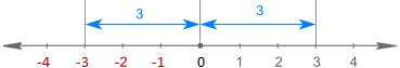 Nilai mutlak dalam Excel: Fungsi ABS dengan contoh formula
Apr 06, 2025 am 09:12 AM
Nilai mutlak dalam Excel: Fungsi ABS dengan contoh formula
Apr 06, 2025 am 09:12 AM
Tutorial ini menerangkan konsep nilai mutlak dan menunjukkan aplikasi Excel praktikal fungsi ABS untuk mengira nilai mutlak dalam dataset. Nombor boleh positif atau negatif, tetapi kadang -kadang hanya nilai positif yang diperlukan
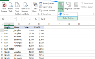 Excel: baris kumpulan secara automatik atau secara manual, runtuh dan mengembangkan baris
Apr 08, 2025 am 11:17 AM
Excel: baris kumpulan secara automatik atau secara manual, runtuh dan mengembangkan baris
Apr 08, 2025 am 11:17 AM
Tutorial ini menunjukkan cara menyelaraskan spreadsheet Excel kompleks dengan mengumpulkan baris, menjadikan data lebih mudah untuk dianalisis. Belajar dengan cepat menyembunyikan atau menunjukkan kumpulan baris dan meruntuhkan keseluruhan garis besar ke tahap tertentu. Hamparan besar dan terperinci boleh
 COUNTIF SPREWEET COUNTIF Google dengan contoh formula
Apr 11, 2025 pm 12:03 PM
COUNTIF SPREWEET COUNTIF Google dengan contoh formula
Apr 11, 2025 pm 12:03 PM
Menguasai sheet google countif: panduan komprehensif Panduan ini meneroka fungsi countif serba boleh di Helaian Google, menunjukkan aplikasinya di luar pengiraan sel mudah. Kami akan merangkumi pelbagai senario, dari perlawanan tepat dan separa ke Han
