

Cara memilih baris dan lajur di Excel

In this article, we will guide you through various methods to select rows and columns in Excel, including some helpful shortcuts.
Efficiency is the name of the game when it comes to Excel. Selecting rows and columns might seem like a small task, but it opens the door to endless possibilities for data transformation and customization.
How to select an entire column in Excel
Selecting an entire column in Excel is simple. Just click on the column header, which displays the letter corresponding to the column, such as A, B or C. By clicking on the header, the entire column will be highlighted, indicating that it is selected.
Alternatively, you can use a keyboard shortcut to select a whole column in Excel:
- Click on any cell within the column.
- Press Ctrl + Spacebar together.

How to select a whole row in Excel
Similar to selecting a column, selecting a whole row in Excel is straightforward. Just click on the row header, which displays the row number, such as 1, 2 or 3. This will highlight the entire row, indicating that it is selected.
An entire row can also be selected with a simple shortcut:
- Click on any cell within the row.
- Press the Shift + Spacebar keys simultaneously.

How to select multiple columns in Excel
To select two or more columns in Excel, you have a few options at your disposal:
Mouse method. Click on the header of the first column you want to select and drag your mouse to the header of the last column. As you do so, all the columns in between will get highlighted.
Shift key. Another quick way to select several adjacent columns is this:
- First, click on the header of the column from where you want to start your selection.
- Then, while holding down the Shift key, click on the header of the column where you want your selection to end.
Keyboard shortcut. To streamline your workflow even further, you can use keyboard shortcut. Select several adjacent cells in one row and press the Ctrl + Space keys simultaneously to select the entire columns.

Tip. When you want to freeze selected rows, keep in mind that Microsoft Excel allows freezing only rows at the top of the spreadsheet. To achieve the effect of freezing specific rows, select the row below the last row you want to freeze, and then utilize the Freeze Panes feature. For a detailed tutorial on how to accomplish this, refer to this article: How to freeze rows in Excel.
Select non-adjacent columns in Excel
To select multiple non-adjacent columns, hold down the Ctrl key on your keyboard while clicking on the headers of the desired columns. Each time you click on a column header, it will be added to your selection.

This method allows you to cherry-pick specific columns from different areas of your worksheet, empowering you to apply operations or formatting exclusively to those chosen columns.
How to select multiple rows in Excel
Selecting multiple rows in Excel is a fundamental skill that allows you to work efficiently with data sets of varying sizes. Let's explore different methods for selecting multiple rows in Excel.
Select adjacent rows
To select multiple contiguous rows, you have a couple of options:
- Click on the header of the first row you wish to select and drag your mouse to the header of the last row.
- An alternative method is to select the first row, then hold down the Shift key while clicking on the header of the last row. This method quickly highlights a range of consecutive rows without the need for dragging the mouse.
- Or you can just select the first cells in the target rows and use Shift + Space shortcut to extend the selection to entire rows.

Select non-adjacent rows
To select individual non-adjacent rows, you can utilize the Ctrl key on your keyboard:
- Hold down the Ctrl key.
- Click on the headers of the desired rows while holding down the Ctrl key. Each row you click will be added to the selection.
This method is useful when you want to perform specific manipulations on specific rows without affecting others.

Select multiple rows using the Name box
In addition to the conventional methods of selecting rows in Excel, there's another handy technique that involves using the Name box.
To select multiple adjacent rows using the Name box, follow these steps:
- Click on the Name box to activate it.
- Enter the reference of the range of rows you want to select. For example, to highlight rows 3 to 10, enter "3:10" into the Name box.
- Press the Enter key.

Tip. In case you have predefined names for specific rows, click on the drop-down arrow in the Name box and select the desired name from the drop-down list.
Select column to end of data
To quickly select a column that extends to the end of the data range, you can use the Ctrl + Shift + Down Arrow keyboard shortcut. Here's how:
- Click on the first cell in the column or on any other cell where you want to start the selection.
- Hold down the Ctrl and Shift keys and then press the Down Arrow key.
This shortcut will select the entire column from your current position to the last cell in the column that contains data.

This technique is especially handy when working with large datasets, as it saves you the effort of manually scrolling and selecting the whole column.
Select all rows below in Excel
The Ctrl + Shift + Down Arrow shortcut can also be used to select all the rows below a certain point in Excel. Here are step-by-step instructions:
- Select the first cell in the row where you want to start the selection.
- Hold down the Shift key and use the Right Arrow key to extend the selection to as many columns as needed.
- Release the Shift key once you have selected all the necessary columns.
- Now, it's time to select all rows below. Press and hold the Ctrl and Shift key simultaneously. While holding down both keys, press the Down Arrow key.
Excel will automatically select all the rows below, from the starting point you selected until the last row of data in your dataset.

Expanding on the same concept, you can select all rows above, to the right, or to the left of a given row using keyboard shortcuts. To achieve this, combine the Up, Right, or Left arrow keys with the Ctrl + Shift shortcut.
For example, to select all rows above, hold Ctrl + Shift + Up Arrow.
Similarly, use Ctrl + Shift + Right Arrow to select all rows to the right and Ctrl + Shift + Left Arrow to select all rows to the left.
These shortcuts provide additional flexibility in selecting rows based on your specific needs, so you can perform calculations or formatting on a subset of data.
Note. Be aware that this method only selects non-empty rows. So, make sure to consider the presence of gaps in your dataset when using this selection technique.
Select columns and rows in Excel table
When working with formatted tables in Excel, you have access to a convenient and intuitive way to select specific columns and rows.
Selecting a column in a table
Selecting an entire column in a table is a breeze with these techniques:
To select a table column, simply hover the mouse cursor over the top edge of the column header. As you do so, a small black selection arrow will appear. Clicking the top edge once will select the column data without the header. If you click it twice, the entire table column, including the header, will be selected. This way, you can highlight either the column's data or the entire column in one or two clicks.

Alternatively, you can click anywhere within the table column and press the Ctrl + Spacebar keys together. Pressing the shortcut once selects the column data, while pressing it twice selects the entire table column along with its header. This way you can accomplish column selection without relying solely on the mouse.
Selecting a row in a table
When it comes to selecting a whole row in a table, Excel offers a similar straightforward technique:
Hover the mouse cursor over the left border of the row until the small black selection arrow appears. This indicator signifies that clicking on the border will select the entire row.

Another option is to click on any cell in a given row, and then press the Shift + Spacebar shortcut. This combination of keys enables you to select the entire row effortlessly, regardless of your current position within the row.
Select rows with certain value in a column
To select all rows that have a specific value in some column, you can use Excel's Filter feature. Follow these steps to filter and select the desired rows:
- Select any cell within your dataset.
- Go to the Data tab and click on the Filter button. This will enable the filter functionality and add filter dropdowns to each column header.
- In the column that contains the specific value you want to filter by, click on the filter arrow and pick the desired value(s) from the drop-down menu. Excel will filter the data and display only the rows that match the selected value.

Once the filtering is applied, you can select the filtered rows using either the mouse or convenient cell selectin shortcuts.

Now that you've successfully selected the rows that meet your criteria, you can perform various actions on them. Copy the selected rows to another location, apply specific formatting, perform calculations, or analyze the data further based on your requirements.
Select rows based on a cell value using Ultimate Suite
If you find yourself unable to apply Excel's Filter due to non-adjacent rows in your sheet or other limitations, don't worry! Our Ultimate Suite offers the Advanced Filter and Replace tool, which is designed to handle such scenarios effortlessly. With this tool, you can search within a specific sheet or across multiple worksheets at a time, allowing you to select found entries or entire rows based on specific criteria.
To select all rows containing a certain value, whether adjacent or non-adjacent, follow these steps:
- Begin by clicking the Find and Replace icon on the Ablebits Tools tab.
- In your worksheet, select the target column where you want to search for the desired value.
- On the Advanced Find and Replace pane, configure your search options:
- Enter the value you wish to search for.
- Choose to search within the selected range.
- Once you have set up your search criteria, click the Find All button.

Once the search is complete, you can proceed to select the desired rows. To do this, click the Select cells button at the bottom of the pane. A drop-down menu will appear, allowing you to choose whether to select entire rows or columns that contain the found entries.

Tip. To select rows that contain a specific value in any column, simply choose to search within the entire sheet. Or select the whole dataset first, and then search within the selection.
This functionality enables you to extract specific data quickly and easily, even in complex scenarios where Excel's native filtering capabilities may fall short.
As you see, Microsoft Excel offers a range of techniques to select entire rows and columns as well as multiple rows based on cell values. So, dive in, explore the various selection methods, and empower yourself to excel in Excel! :)
Atas ialah kandungan terperinci Cara memilih baris dan lajur di Excel. Untuk maklumat lanjut, sila ikut artikel berkaitan lain di laman web China PHP!

Alat AI Hot

Undresser.AI Undress
Apl berkuasa AI untuk mencipta foto bogel yang realistik

AI Clothes Remover
Alat AI dalam talian untuk mengeluarkan pakaian daripada foto.

Undress AI Tool
Gambar buka pakaian secara percuma

Clothoff.io
Penyingkiran pakaian AI

Video Face Swap
Tukar muka dalam mana-mana video dengan mudah menggunakan alat tukar muka AI percuma kami!

Artikel Panas
Alat panas

Notepad++7.3.1
Editor kod yang mudah digunakan dan percuma

SublimeText3 versi Cina
Versi Cina, sangat mudah digunakan

Hantar Studio 13.0.1
Persekitaran pembangunan bersepadu PHP yang berkuasa

Dreamweaver CS6
Alat pembangunan web visual

SublimeText3 versi Mac
Perisian penyuntingan kod peringkat Tuhan (SublimeText3)
Topik panas
 1653
1653
 14
1413
52
1304
25
1251
29
1224
24
14
1413
52
1304
25
1251
29
1224
24

 Cara Menambah Kalendar Ke Outlook: Dikongsi, Kalendar Internet, Fail ICAL
Apr 03, 2025 am 09:06 AM
Cara Menambah Kalendar Ke Outlook: Dikongsi, Kalendar Internet, Fail ICAL
Apr 03, 2025 am 09:06 AM
Artikel ini menerangkan cara mengakses dan menggunakan kalendar bersama dalam aplikasi desktop Outlook, termasuk mengimport fail icalendar. Sebelum ini, kami meliputi berkongsi kalendar Outlook anda. Sekarang, mari kita meneroka bagaimana melihat kalendar yang dikongsi bersama
 Cara menggunakan flash isi excel dengan contoh
Apr 05, 2025 am 09:15 AM
Cara menggunakan flash isi excel dengan contoh
Apr 05, 2025 am 09:15 AM
Tutorial ini menyediakan panduan komprehensif untuk ciri pengisian kilat Excel, alat yang berkuasa untuk mengautomasikan tugas kemasukan data. Ia meliputi pelbagai aspek, dari definisi dan lokasinya untuk penggunaan dan penyelesaian masalah lanjutan. Memahami Fla Excel
 Formula Median di Excel - Contoh Praktikal
Apr 11, 2025 pm 12:08 PM
Formula Median di Excel - Contoh Praktikal
Apr 11, 2025 pm 12:08 PM
Tutorial ini menerangkan cara mengira median data berangka dalam Excel menggunakan fungsi median. Median, ukuran utama kecenderungan pusat, mengenal pasti nilai pertengahan dalam dataset, yang menawarkan perwakilan yang lebih mantap dari Tenden Central
 Buku Kerja Dikongsi Excel: Cara berkongsi fail Excel untuk beberapa pengguna
Apr 11, 2025 am 11:58 AM
Buku Kerja Dikongsi Excel: Cara berkongsi fail Excel untuk beberapa pengguna
Apr 11, 2025 am 11:58 AM
Tutorial ini menyediakan panduan komprehensif untuk berkongsi buku kerja Excel, meliputi pelbagai kaedah, kawalan akses, dan resolusi konflik. Versi Excel Moden (2010, 2013, 2016, dan kemudian) Memudahkan pengeditan kolaboratif, menghapuskan keperluan untuk m
 Cara mengeja daftar masuk excel
Apr 06, 2025 am 09:10 AM
Cara mengeja daftar masuk excel
Apr 06, 2025 am 09:10 AM
Tutorial ini menunjukkan pelbagai kaedah untuk pemeriksaan ejaan dalam Excel: cek manual, makro VBA, dan menggunakan alat khusus. Belajar untuk memeriksa ejaan dalam sel, julat, lembaran kerja, dan seluruh buku kerja. Walaupun Excel bukan pemproses kata, spelnya
 Nilai mutlak dalam Excel: Fungsi ABS dengan contoh formula
Apr 06, 2025 am 09:12 AM
Nilai mutlak dalam Excel: Fungsi ABS dengan contoh formula
Apr 06, 2025 am 09:12 AM
Tutorial ini menerangkan konsep nilai mutlak dan menunjukkan aplikasi Excel praktikal fungsi ABS untuk mengira nilai mutlak dalam dataset. Nombor boleh positif atau negatif, tetapi kadang -kadang hanya nilai positif yang diperlukan
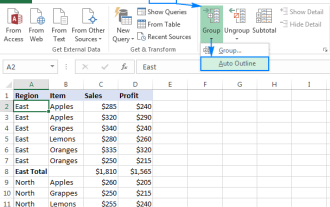 Excel: baris kumpulan secara automatik atau secara manual, runtuh dan mengembangkan baris
Apr 08, 2025 am 11:17 AM
Excel: baris kumpulan secara automatik atau secara manual, runtuh dan mengembangkan baris
Apr 08, 2025 am 11:17 AM
Tutorial ini menunjukkan cara menyelaraskan spreadsheet Excel kompleks dengan mengumpulkan baris, menjadikan data lebih mudah untuk dianalisis. Belajar dengan cepat menyembunyikan atau menunjukkan kumpulan baris dan meruntuhkan keseluruhan garis besar ke tahap tertentu. Hamparan besar dan terperinci boleh
 COUNTIF SPREWEET COUNTIF Google dengan contoh formula
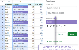
Apr 11, 2025 pm 12:03 PM
COUNTIF SPREWEET COUNTIF Google dengan contoh formula
Apr 11, 2025 pm 12:03 PM
Menguasai sheet google countif: panduan komprehensif Panduan ini meneroka fungsi countif serba boleh di Helaian Google, menunjukkan aplikasinya di luar pengiraan sel mudah. Kami akan merangkumi pelbagai senario, dari perlawanan tepat dan separa ke Han
